Notes on concordance
Motivation
I don’t understand the details of concordance in survival analysis, so I’m trying to explain it to myself.
Probabilistic index
I recently read the very nice paper On the interpretation of the hazard ratio in Cox regression by Jan De Neve and Thomas Gerds.
Suppose in the context of a clinical trial we use a Cox model to compare an experimental treatment (A=1) with a control treatment (A=0), where (for simplicity here) treatment is the only term in the model (assume the model is correct, by the way). Let \(\theta\) denote the hazard ratio.
De Neve and Gerds recommend interpreting the treatment effect as a probabilistic index, that is, the probability that a randomly chosen patient on the experimental arm has a survival time (\(T_{1,j}\)) that is longer than the survival time (\(T_{0,i}\)) for a randomly chosen patient on the control arm . They show that:
\[P(T_{0,i} < T_{1,j}) = \frac{1}{1 + \theta}.\]
That’s a super interesting relationship. However, they only show a proof for uncensored data. How should we interpret the probabilistic index in a trial with a maximum follow-up time and administrative right censoring (i.e. almost every trial)?
In their discussion, De Neve and Gerds say that we must assume proportional hazards also holds after the maximum follow up time. This suggests that when interpreting \(P(T_{0,i} < T_{1,j})\), we are indeed thinking about an infinite follow-up.
This makes me slightly uncomfortable. We can check (to some extent) whether proportional hazards looks like a reasonable assumption for the duration of the study. Assuming it continues to hold until all patients have had their event is a bit more of a stretch. It got me wondering: does the following relationship still hold:
\[P(T_{0,i} < T_{1,j} \mid \text{It's possible to know given censoring}) = \frac{1}{1 + \theta}?\]
How can I formulate that a bit more precisely? Denote the censoring times for patients \(i\) and \(j\) as \(C_{0,i}\) and \(C_{1,j}\) (and assume, by the way, that censoring and survival distributions are independent). In order to know for sure whether or not \(T_{0,i} < T_{1,j}\), I need the minimum of \(T_{1,j}\) and \(T_{0,i}\) to be uncensored. Also, if the maximum of \(T_{1,j}\) and \(T_{0,i}\) is censored, I at least need the censoring time to come after the minimum of \(T_{1,j}\) and \(T_{0,i}\). So, having picked two patients at random, in order to establish who has the better survival time I need \(\min\{T_{0,i},T_{1,j}\} < \min\{C_{0,i}, C_{1,j} \}\). My question becomes: does
\[P(T_{0,i} < T_{1,j} \mid \min\{T_{0,i},T_{1,j}\} < \min\{C_{0,i}, C_{1,j} \} ) = \frac{1}{1 + \theta}?\]
Is the answer obvious? I have a bad feeling it might be and I’m about to do some unnecessary, tedious maths. I’ll condition on the censoring times. Let \(\tau:= \min\{C_{0,i}, C_{1,j}\}\). I’m interested in
\[ \begin{aligned} P(T_{0,i} < T_{1,j} \mid \min\{T_{0,i},T_{1,j}\} < \tau ) & = P(T_{0,i} < T_{1,j} \mid T_{0,i} < \tau \cup T_{1,j} < \tau ) \\ & = \frac{P(T_{0,i} < T_{1,j} \cap T_{0,i} < \tau )}{ P( T_{0,i} < \tau \cup T_{1,j} < \tau )} \\ \end{aligned} \]
where I have used the fact that if \(T_{1,j} < \tau\) but \(T_{0,j} > \tau\), then it is impossible for \(T_{0,i} < T_{1,j}\). Starting with the numerator, I apply the survival distribution \(S_1\) to everything:
\[ \begin{aligned} P(T_{0,i} < T_{1,j} \cap T_{0,i} < \tau )& = P(S_1(T_{0,i}) > S_1(T_{1,j}) \cap S_1(T_{0,i}) > S_1(\tau) )\\ &= P(S_0(T_{0,i})^\theta > S_1(T_{1,j}) \cap S_0(T_{0,i})^\theta > S_1(\tau) )\\ &= P(U_0^\theta > U_1 \cap U_0 > u_*^{1/\theta} ) \end{aligned} \] where I have used proportional hazards, \(S_1(t)=S_0(t)^\theta\) for \(t \in (0,\tau)\), and defined \(U_0 = S_0(T_{0,i})\), \(U_1 = S_1(T_{1,i})\), and \(u_*=S_1(\tau)\). Since \(U_0\) and \(U_1\) are independent uniform, we have
\[ \begin{aligned} P(U_0^\theta > U_1 \cap U_0 > u_*^{1/\theta} ) &= \int_{u_*^{1/\theta}}^1 u_0^\theta du_0 \\ &= \left[ \frac{u_0^{\theta+1}}{\theta+1} \right]_{u_*^{1/\theta}}^1 \\ &= \frac{1 - u_*^{1+\frac{1}{\theta}}}{\theta + 1} \end{aligned} \]
Similarly for the denominator, \[ \begin{aligned} P( T_{0,i} < \tau \cup T_{1,j} < \tau )& = P( S_1(T_{0,i}) > S_1(\tau) \cup S_1(T_{1,j}) > S_1(\tau) )\\ &= P( S_0(T_{0,i})^{\theta} > S_1(\tau) \cup S_1(T_{1,j}) > S_1(\tau) ) \\ &= P( U_0 > u_*^{1/\theta} \cup U_1 > u_* )\\ &= 1 - P( U_0 < u_*^{1/\theta} \cap U_1 < u_* ) \\ &= 1 - u_*^{1+\frac{1}{\theta}}, \end{aligned} \] and dividing the numerator by the denominator finally gives the result that \[ P(T_{0,i} < T_{1,j} \mid \min\{T_{0,i},T_{1,j}\} < \min\{C_{0,i}, C_{1,j} \} ) = \frac{1}{1 + \theta}. \] Maybe this was overkill. But it’s settled my mind a little. If someone tells me that the probabilistic index is \(\phi=1/(1+\theta)\) (in the context of a proportional hazards model applied to a particular trial with administrative censoring), then I can imagine repeatedly selecting two patients at random, one from each arm. Out of the pairs where it is possible to establish who has better survival, the fraction of times that it is the patient from the experimental arm is \(\phi\).
[As an aside, I much prefer the interpretation \(S_1(t)=S_0(t)^\theta\) as the interpretation of the hazard ratio. Looking at the above derivation, this is the more fundamental relationship. But, then again, there are several interpretations of the hazard ratio, each with pros and cons…would need a separate post.]
Link with concordance
I can try to show an example using the concordance() function from R’s survival package. Firstly, I set up a data frame with some exponentially distributed survival data from a clinical trial. The control arm median is 12 months. The experimental arm median is 18 months. Recruitment is uniform over 12 months. The sample size of 5000 per arm is deliberately oversized for illustration purposes (so the point estimate of the hazard ratio is close to 0.66).
library(dplyr)
library(survival)

set.seed(325)

df_ex <- data.frame(rec = runif(10000, 0, 12),
                    y_star = c(rexp(5000, rate = log(2) / 12),
                               rexp(5000, rate = log(2) / 18)),
                    delta_star = 1,
                    trt = rep(c("0", "1"), each = 5000)) %>%
   mutate(delta = as.numeric(y_star + rec < 18),
          y = pmin(y_star, 18 - rec))

head(df_ex)
## rec y_star delta_star trt delta y
## 1 3.4275172 15.893085 1 0 0 14.572483
## 2 9.3391460 8.595456 1 0 1 8.595456
## 3 2.1307085 9.754036 1 0 1 9.754036
## 4 2.1295279 8.575436 1 0 1 8.575436
## 5 0.6061914 4.822211 1 0 1 4.822211
## 6 6.3240452 4.126706 1 0 1 4.126706The data frame contains two versions of the data set. (y_star, delta_star) is the survival time and event status (1=event; 0=censored) for the uncensored data set, assuming an infinite follow-up time. (y, delta) is the survival time and event status, assuming administrative censoring 18 months after the start of the study. I can quickly plot (without tidying up axis labels etc) the Kaplan Meier estimates for the two data sets:
fit_inf <- survfit(Surv(y_star, delta_star) ~ trt, data = df_ex)
fit_18 <- survfit(Surv(y, delta) ~ trt, data = df_ex)

plot(fit_inf, col = 1:2)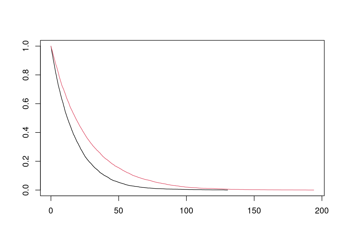
plot(fit_18, col = 1:2)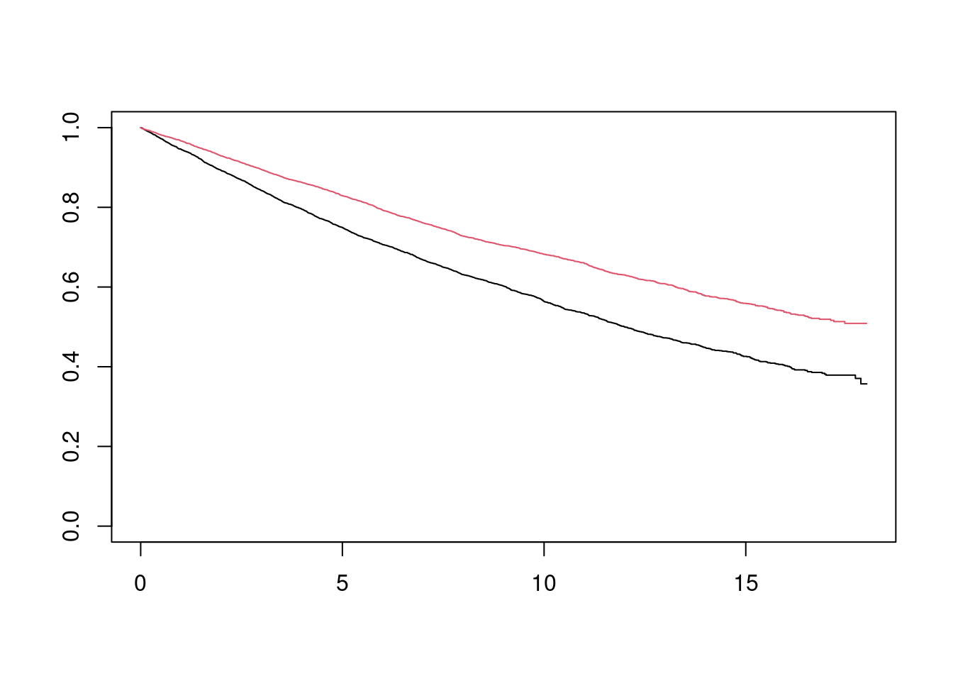
I’ll start with the infinite follow-up data set, and fit a Cox model to confirm that the hazard ratio is essentially 0.66…
cph_inf <- coxph(Surv(y_star, delta_star) ~ trt, data = df_ex)
summary(cph_inf)$coef
## coef exp(coef) se(coef) z Pr(>|z|)
## trt1 -0.4197819 0.6571902 0.02043946 -20.53781 9.891931e-94I could then estimate the probabilistic index as \(1/(1+0.66)= 0.6\).
Next I calculate the concordance…
con_inf <- concordance(cph_inf)
con_inf
## Call:
## concordance.coxph(object = cph_inf)
##
## n= 10000
## Concordance= 0.5505 se= 0.002813
## concordant discordant tied.x tied.y tied.xy
## 15025449 9974551 24995000 0 0We see that the concordance is 0.55. So concordance is not the same as the probabilistic index.
What is concordance?
See this nice vignette by Thernau & Atkinson. The motivation for concordance usually comes from evaluating the performance of a risk prediction model, rather than quantifying treatment effect. It was proposed in this context by Frank Harrell in this 1982 paper. The idea is that if I randomly select two patients from the entire population, what is the probability that the model prediction agrees with reality in terms of who has the longer survival time? Loosely speaking, concordance is defined as \[ P(\hat{T}_i < \hat{T}_j \mid T_{i} < T_{j}), \] and if there were no ties, this would be the same as \[ P(T_i < T_j \mid \hat{T}_i < \hat{T}_j). \] It’s just saying that, out of all possible samples of size 2 from the whole population, how often does the actual ordering of events match the predicted ordering. However, to deal with ties, the definition of concordance is typically extended to \[ \begin{align} \text{Concordance}:&=P( \hat{T}_i < \hat{T}_j \mid T_i < T_j, \hat{T}_i\neq \hat{T}_j)P(\hat{T}_i \neq \hat{T}_j\mid T_i \neq T_j) + \frac{1}{2}P(\hat{T}_i = \hat{T}_j \mid T_i \neq T_j),\\ \end{align} \] or, equivalently, \[ P(T_i < T_j \mid \hat{T}_i < \hat{T}_j, T_i \neq T_j)P(\hat{T}_i \neq \hat{T}_j \mid T_i \neq T_j) + \frac{1}{2}P(\hat{T}_i = \hat{T}_j \mid T_i \neq T_j). \]
This is just saying that, out of all samples of size 2 from the whole population, if we discard samples with tied events, how often can we correctly predict from the model who will have the longer survival times (where if our model gives us tied predictions then we choose randomly / are correct with probability 0.5)?
In our clinical trial context, and for our first simulated data set where there are no ties in \(T\) and no censoring, we have \[ \begin{align} \text{Concordance}&=P(T_i < T_j \mid A_i = 0, A_j = 1)P(A_i \neq A_j) + \frac{1}{2}P(A_i = A_j)\\ &= \text{Probabilistic Index } \times P(A_i \neq A_j) + \frac{1}{2}P(A_i = A_j). \end{align} \]
Since \(P(A_i = A_j)\) is just telling us the allocation ratio, the Concordance and Probabilistic Index are essentially carrying the same information about the treatment effect. The Probabilistic Index is more natural for describing a treatment effect. Concordance is more natural for describing performance of a risk prediction model.
Going back to our example
con_inf## Call:
## concordance.coxph(object = cph_inf)
##
## n= 10000
## Concordance= 0.5505 se= 0.002813
## concordant discordant tied.x tied.y tied.xy
## 15025449 9974551 24995000 0 0the concordance() function has helpfully provided us with the number of concordant, discordant and tied.x pairs. From these, we can get empirical estimates for both the probabilistic index and the concordance. The total number of pairs is choose(10000,2) = 49,995,000. The number of pairs where both patients are on the same treatment arm is 2*choose(5000,2) = 24,995,000. That’s what we see in tied.x. We have 5000 * 5000 = 25,000,000 pairs where one patient comes from each arm. Of these, we see that 15,025,449 are concordant, meaning that the survival of the patient on the experimental arm was longer than the survival of the patient on the control arm, and the rest were discordant. So an empirical estimate for the probabilistic index is 15,025,449 / 25,000,000 = 0.60, which agrees with our theoretical result above. And the empirical estimate for the concordance is
\[ \frac{15,025,449}{25,000,000}\times\frac{25,000,000}{49,995,000} + 0.5 \times \frac{24,995,000}{49,995,000} = 0.550514, \] which is exactly what we see.
Now let’s move on to the censored data set…
cph_18 <- coxph(Surv(y, delta) ~ trt, data = df_ex)
summary(cph_18)$coef
## coef exp(coef) se(coef) z Pr(>|z|)
## trt1 -0.3942244 0.6742028 0.03099125 -12.7205 4.549172e-37In this case everything looks the same…
con_18 <- concordance(cph_18)
con_18
## Call:
## concordance.coxph(object = cph_18)
##
## n= 10000
## Concordance= 0.5495 se= 0.004008
## concordant discordant tied.x tied.y tied.xy
## 9023362 6051734 14914532 0 0except that all pairs where it is impossible to establish for certain which patient had the longer survival time have been removed from consideration, and hence we see lower numbers of concordant, discordant and tied.x pairs. An empirical estimate of the probabilistic index, which remember I defined as
\[P(T_{0,i} < T_{1,j} \mid \text{It's possible to know given censoring})\]
is concordant / (concordant + discordant) = 9023362 / (9023362 + 6051734) = 0.60, mathching the theoretical result.
For the concordance, I also need to modify the definition. Let \(E_{i,j}\) denote the event “It’s possible to know which of \(T_i\) and \(T_j\) happens first”. Then
\[ \text{Concordance}:=P(T_i < T_j \mid \hat{T}_i < \hat{T}_j, T_i \neq T_j,E_{i,j})P(\hat{T}_i \neq \hat{T}_j \mid T_i \neq T_j,E_{i,j}) + \frac{1}{2}P(\hat{T}_i = \hat{T}_j \mid T_i \neq T_j,E_{i,j}). \] I can estimate this empirically as
\[ \frac{9023362}{9023362 + 6051734}\times\frac{9023362 + 6051734}{9023362 + 6051734 + 14914532} + 0.5 \times \frac{14914532}{9023362 + 6051734 + 14914532} = 0.5495443, \]
which is exactly what we see.
Further Topics
I wanted to explain a bit more about
- standard errors for concordance. Both for empirical estimates. And using the reationship with the hazard ratio.
- alternative weighted versions of concordance (see the vignette)
- a non-proportional hazards example.
But I’ve run out of steam. Maybe I’ll come back to it another time.
P.S. standard errors
Follows (https://cran.r-project.org/web/packages/survival/vignettes/concordance.pdf) closely.
Let’s take the same example as before, except we reduce the sample size from 10,000 to 400 so that it makes sense to worry about standard errors.
library(dplyr)
library(survival)

set.seed(325)

df_ex <- data.frame(rec = runif(400, 0, 12),
                    y_star = c(rexp(200, rate = log(2) / 12),
                               rexp(200, rate = log(2) / 18)),
                    delta_star = 1,
                    trt = rep(c("0", "1"), each = 200)) %>%
   mutate(delta = as.numeric(y_star + rec < 18),
          y = pmin(y_star, 18 - rec))

head(df_ex)
## rec y_star delta_star trt delta y
## 1 3.4275172 39.246498 1 0 0 14.572483
## 2 9.3391460 25.012807 1 0 0 8.660854
## 3 2.1307085 1.414864 1 0 1 1.414864
## 4 2.1295279 12.747489 1 0 1 12.747489
## 5 0.6061914 17.157924 1 0 1 17.157924
## 6 6.3240452 10.810010 1 0 1 10.810010fit_inf <- survfit(Surv(y_star, delta_star) ~ trt, data = df_ex)
fit_18 <- survfit(Surv(y, delta) ~ trt, data = df_ex)
plot(fit_inf, col = 1:2)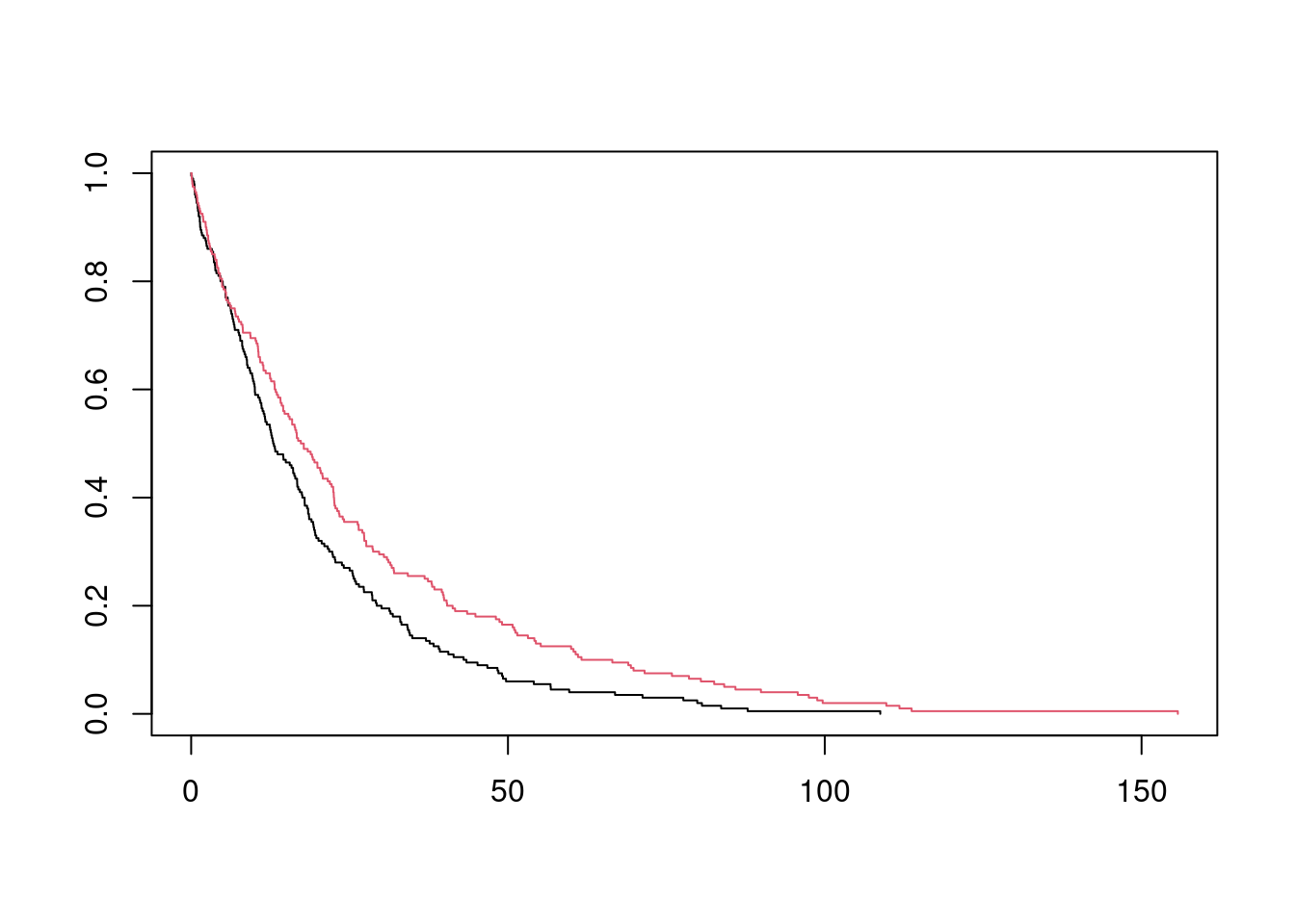
plot(fit_18, col = 1:2)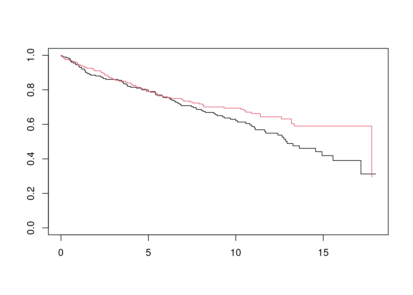
Confidence interval for Probabilistic Index using the relationship \(\phi = 1 / (1 + \theta)\)
## Infinite follow-up
cph_inf <- coxph(Surv(y_star, delta_star) ~ trt, data = df_ex)

## Point estimate
1 / (1 + exp(cph_inf$coefficients))
## trt1
## 0.5793188## CI
rev(1 / (1 + exp(confint(cph_inf))))## [1] 0.5299843 0.6271182## 18 month max follow-up
cph_18 <- coxph(Surv(y, delta) ~ trt, data = df_ex)
## Point estimate
1 / (1 + exp(cph_18$coefficients))## trt1
## 0.5730088## CI
rev(1 / (1 + exp(confint(cph_18))))## [1] 0.4958763 0.6467470Standard error of concordance (empirical)
The standard error for the empirical estimator of the concordance can be calculated based on the nice observation by Therneau and Watson that a standardized version of this estimator is equal to the score statistic from a Cox model with a time-dependent covariate \(n(t_i)r_i(t_i)\), where \(n(t_i)\) and \(r_i(t_i)\) are defined as ” the number of subjects still at risk at time t” and “the rank of \(x_i\) among all those still at risk at time \(t\)”, respectively. I found it quite difficult to get my head around the exact definition of \(n(t_i)\) and \(r_i(t_i)\), and also to understand why there is this equivalence. To avoid that pain again, I’ll now try to explain in excessive detail…
Starting with the empirical estimate for concordance:
\[ \tilde{C} = \frac{\sum_{\text{pairs}: E_{i,j}\cap (T_i < T_j)} I(\hat{T}_i<\hat{T}_j)+ 0.5I(\hat{T}_i<\hat{T}_j)}{\sum_{\text{pairs}: E_{i,j}\cap (T_i < T_j) } I(\hat{T}_i<\hat{T}_j) + I(\hat{T}_i>\hat{T}_j) + I(\hat{T}_i=\hat{T}_j)}\]
where \(E_{i,j}\) is the event that it’s possible to establish which of \(T_i\) and \(T_j\) is larger given censoring, we can then rearrange:
\[ \left\lbrace \sum_{\text{pairs}: E_{i,j}\cap (T_i < T_j)} 1 \right\rbrace \left( 2\tilde{C}-1 \right) = \sum_{\text{pairs}: E_{i,j}\cap (T_i < T_j)} I(\hat{T}_i<\hat{T}_j) - I(\hat{T}_i>\hat{T}_j) =: U.\]
The next step is to recognize that we can sum up the terms in \(U\) in a particular order:
\[ U = \sum_i \sum_{j: E_{i,j} \cap (T_j > T_i)} \text{sign}(\hat{T}_j - \hat{T}_i)\] where \(\text{sign}(z)\)=-1,0 or 1, depending if \(z\) is \(<0\), \(=0\) or \(>0\).
For a pair \((i,j)\) to satisfy \(E_{i,j} \cap (T_j > T_i)\), we firstly need the survival time \(T_i\) to be uncensored. Also, we need patient \(j\) to be in the at-risk set at time \(T_i\). This is sufficient to satisfy the condition. So we have
\[U = \sum_i \delta_i \sum_{j: j\neq i,j\in R(T_i) } \text{sign}(\hat{T}_j - \hat{T}_i),\]
where \(\delta_i\) is an indicator that patient \(i\) has an event, and \(R\) denotes the risk set. The same expression is found in Appendix A of Therneau and Watson. At this point, we can introduce the more precise definitions for \(r_i(t_i)\) and \(n(t_i)\):
\[r_i(t_i):= \frac{1}{n(t_i)}\sum_{j: j\neq i,j\in R(T_i)} \left[ I(\hat{T}_i < \hat{T}_j) + \frac{1}{2}I(\hat{T}_i = \hat{T}_j)\right], \] where \(n(t_i):= |j: j\neq i,j\in R(T_i)|\), i.e., the size of the risk set (excluding \(i\) itself). Next (following T&W),
\[ \begin{align} r_i(t_i) &= \frac{1}{n(t_i)}\sum_{j: j\neq i,j\in R(T_i)} \left[ I(\hat{T}_i < \hat{T}_j) + \frac{1}{2}I(\hat{T}_i = \hat{T}_j)\right]\\ &= \frac{1}{n(t_i)}\sum_{j: j\neq i,j\in R(T_i)} \left[ \text{sign}(\hat{T}_j - \hat{T}_i) + 1 \right] /2\\ &= \frac{1}{2} + \frac{1}{n(t_i)}\sum_{j: j\neq i,j\in R(T_i)} \frac{\text{sign}(\hat{T}_j - \hat{T}_i)}{2} \end{align} \]
and therefore
\[U = \sum_i 2\delta_i n(t_i)\{r_i(t_i) - 1 / 2\}\]
To see that this is equivalent to a Cox model, we must further recognize that \(\bar{r} = 1/2\), where \(\bar{r}\) is the average of the \(r_i\) across all \(i\) at risk at time \(t_i\) (this is because the \(j\neq i\) terms cancel each other out), and finally write down the partial likelihood from the Cox model with a time-dependent covariate \(z(t)\):
\[\sum_i \delta_i \left[ z_i(t_i) - \frac{\sum_{j \in R(t_i)} z_j(t_i) \exp\left[ z_j(t_i)\beta \right]}{\exp\left[ z_j(t_i)\beta \right]} \right] \mid_{\beta = 0} = \sum_i \delta_i \left[ z_i(t_i) - \bar{z}(t_i)\right],\]
observing the equivalence between this expression and the expression for \(U\) when \(z_i(t_i) =2 n(t_i)r_i(t_i)\).
A nice consequence of using the Cox model is that we can write down the variance of this statistic under the null hypothesis (see, e.g., page 128 of https://www4.stat.ncsu.edu/~dzhang2/st745/chap6.pdf):
\[ \sum_i \delta_i \left[ \sum_{j \in R(t_i)} \frac{z_j(t_i)^2}{n(t_i)} - \bar{z}(t_i)^2 \right].\] In principle, I think this is enough to be able to calculate the variance for the empirical estimate of concordance for a general Cox model, but I can’t be bothered any more to actually go through a more complicated example (i.e. a Cox model with more than one variable).
In the context of just two predictions (e.g. in a simple RCT with \(A=0\) and \(A=1\)), the score statistic reduces to the Gehan-Wilcoxon statistic (this is also shown in the appendix of https://www.mayo.edu/research/documents/bsi-techreport-85/doc-20433003)
\[ U= \sum_k n_k (d_{1,k} - \frac{n_{1,k}}{n_1}) \]
with variance
\[\text{var}({U}) = \sum_kn_{k}^2 \times\text{var}\left(d_{1,k} - \frac{n_{1,k}}{n_1}\right)\].
And from these formulas I can reconstruct the estimate of the variance for our example.
The terms \(\{2r_i(t_i) - 1\}\) are guaranteed to be between \(-1\) and \(1\), and they are provided in the rank column by survival::concordance, if we explicitly ask for it:
con_inf <- concordance(cph_inf, ranks = TRUE)
head(con_inf$ranks)
## time rank timewt casewt variance
## 98 0.01382162 0.5012531 399 1 0.2500000
## 313 0.06709051 -0.5000000 398 1 0.2499984
## 257 0.09001529 -0.5012594 397 1 0.2500000
## 40 0.12598446 0.5000000 396 1 0.2499984
## 395 0.14877580 -0.5012658 395 1 0.2500000
## 262 0.18041986 -0.5025381 394 1 0.2499984tail(con_inf$ranks)## time rank timewt casewt variance
## 332 98.80991 -0.1666667 6 1 0.1224490
## 348 99.66819 -0.2000000 5 1 0.1388889
## 164 108.75980 1.0000000 4 1 0.1600000
## 368 109.71749 0.0000000 3 1 0.0000000
## 205 111.79013 0.0000000 2 1 0.0000000
## 396 113.71013 0.0000000 1 1 0.0000000Next I print out the concordance again…
con_inf## Call:
## concordance.coxph(object = cph_inf, ranks = TRUE)
##
## n= 400
## Concordance= 0.5331 se= 0.01436
## concordant discordant tied.x tied.y tied.xy
## 22640 17360 39800 0 0…and show I can reproduce it from the formula above for \(U\) based on \(r\) and \(n\) (79800 is the total number of pairs)…
(sum(con_inf$ranks[,"rank"] * con_inf$ranks[,"timewt"]) / 79800 + 1) / 2## [1] 0.5330827…and I can reproduce the variance for the specific case of just two groups
con_inf$cvar## [1] 0.0002092043(sum((con_inf$ranks["timewt"] + 1) ^2 * con_inf$ranks["variance"])) / (79800^2) / 4## [1] 0.0002092043Still to do
- jacknife estimate of variance
- weighted version of concordance
- non-proportional hazards
I don’t think I’ll get round to this now. Refer to https://www.mayo.edu/research/documents/bsi-techreport-85/doc-20433003
References
De Neve, Jan, and Thomas A. Gerds. “On the interpretation of the hazard ratio in Cox regression.” Biometrical Journal 62.3 (2020): 742-750.
Harrell, Frank E., et al. “Evaluating the yield of medical tests.” Jama 247.18 (1982): 2543-2546.
Therneau, Terry, and Elizabeth Atkinson. “1 The concordance statistic.” (2020).
Dominic Magirr
Medical Statistician
Interested in the design, analysis and interpretation of clinical trials.