Confidence interval for a survival curve based on a Cox model
A colleague caught me out recently when they asked about a confidence interval for a survival curve based on a Cox model. This can be done in R using survival::survfit after survival::coxph. But the question was: does this take into account the uncertainty in the baseline hazard. I had to admit that I wasn’t 100% sure. So here is an example to clear it up…
1. Understanding survfit.coxph standard errors
Create a toy data set and apply survfit.coxph
library(survival)
### create a toy data set
df <- data.frame(time = c(3,5,7,12,17,19,25,26,30),
                 event = rep(1,9),
                 trt = factor(c("A","B","A","B","A","B","A","B","A")))


fit_cox <- coxph(Surv(time, event) ~ trt, data = df)
surv_cox <- survfit(fit_cox, newdata = data.frame(trt = c("A", "B")))
Can I reproduce the estimates and standard errors?
Here are the estimates of survival and std.err (of something) I would like to reproduce in order to understand how they were calculated. The first column corresponds to trt=="A" and the second column to trt=="B"…
surv_cox$surv## 1 2
## [1,] 0.90379995 0.88376336
## [2,] 0.80760960 0.77025266
## [3,] 0.70882912 0.65677247
## [4,] 0.61007108 0.54677825
## [5,] 0.50768592 0.43685968
## [6,] 0.40537172 0.33184585
## [7,] 0.29719960 0.22711842
## [8,] 0.18948065 0.13105127
## [9,] 0.06970604 0.03862672surv_cox$std.err## [,1] [,2]
## [1,] 0.1072286 0.1313337
## [2,] 0.1709941 0.2049614
## [3,] 0.2351795 0.2853216
## [4,] 0.3095973 0.3685374
## [5,] 0.3930877 0.4799235
## [6,] 0.5054737 0.6046534
## [7,] 0.6435328 0.8159658
## [8,] 0.8908094 1.0923455
## [9,] 1.3392316 2.1694201Step 1: Estimate the baseline cumulative hazard
This uses Breslow’s estimator (see slide 39 of https://www.uio.no/studier/emner/matnat/math/STK4080/h16/undervisningsmateriell/lecture8_16.pdf)
The Cox model \(h_0(t)\exp(x\beta)\) has been parameterized in such a way that \(x=0\) corresponds to trt=="A" and \(x=1\) corresponds to trt=="B".
beta_hat <- fit_cox$coef
df$x <- ifelse(df$trt == "B",  1, 0)
df$exp_b <- exp(df$x * beta_hat)
## See formula for Breslow estimator:
H_0 <- cumsum(1 / rev(cumsum(rev(df$exp_b))))
H_0
## [1] 0.1011472 0.2136765 0.3441408 0.4941798 0.6778923 0.9029508 1.2133513
## [8] 1.6634684 2.6634684Note I could instead have used the basehaz function:
basehaz(fit_cox)## hazard time
## 1 0.1011472 3
## 2 0.2136765 5
## 3 0.3441408 7
## 4 0.4941798 12
## 5 0.6778923 17
## 6 0.9029508 19
## 7 1.2133513 25
## 8 1.6634684 26
## 9 2.6634684 30Step 2: Transform to estimated survival curve
### For trt == "A"
exp(-H_0)
## [1] 0.90379995 0.80760960 0.70882912 0.61007108 0.50768592 0.40537172 0.29719960
## [8] 0.18948065 0.06970604## this matches
surv_cox$surv[,1]## [1] 0.90379995 0.80760960 0.70882912 0.61007108 0.50768592 0.40537172 0.29719960
## [8] 0.18948065 0.06970604### For trt == "B"
### the cumulative hazard is equal to the baseline
### cumulative hazard muliplied by exp(beta)
exp(-H_0 * exp(beta_hat))## [1] 0.88376336 0.77025266 0.65677247 0.54677825 0.43685968 0.33184585 0.22711842
## [8] 0.13105127 0.03862672## this matches:
surv_cox$surv[,2]## [1] 0.88376336 0.77025266 0.65677247 0.54677825 0.43685968 0.33184585 0.22711842
## [8] 0.13105127 0.03862672Step 3: Variance of Breslow’s estimator
The variance of Breslow’s estimator is somewhat complicated. It is given on slide 47 of https://www.uio.no/studier/emner/matnat/math/STK4080/h16/undervisningsmateriell/lecture8_16.pdf
And here I just implement their result:
## see definition of s_0 and s_1 in slides:
s_0 = rev(cumsum(rev(df$exp_b)))
s_1 = rev(cumsum(rev(df$exp_b) * rev(df$x)))

var_beta <- c(fit_cox$var)

var_breslow <- var_beta * cumsum(s_1 / s_0 ^ 2) ^ 2 + cumsum(1 / s_0 ^ 2)

## Note that...
sqrt(var_breslow)
## [1] 0.1072286 0.1709941 0.2351795 0.3095973 0.3930877 0.5054737 0.6435328
## [8] 0.8908094 1.3392316## ... already matches
surv_cox$std.err[,1]## [1] 0.1072286 0.1709941 0.2351795 0.3095973 0.3930877 0.5054737 0.6435328
## [8] 0.8908094 1.3392316So the $.std.err given in survfit.coxph is reporting the standard error of the cumulative hazard. When trt=="A" this is the same as the standard error of the baseline cumulative hazard.
To get the standard error when trt=="B", note that the cumulative hazard on treatment B is equal to the baseline cumulative hazard multiplied by \(\exp(\beta)\). So we have to use the delta method, taking into account the variance of the breslow estimator, the variance of beta_hat, and their covariance.
This is messy.
To find their covariance, we use the formulas from https://www.uio.no/studier/emner/matnat/math/STK4080/h16/undervisningsmateriell/lecture8_16.pdf again, where they use the notation \(A\) for the cumulative hazard:
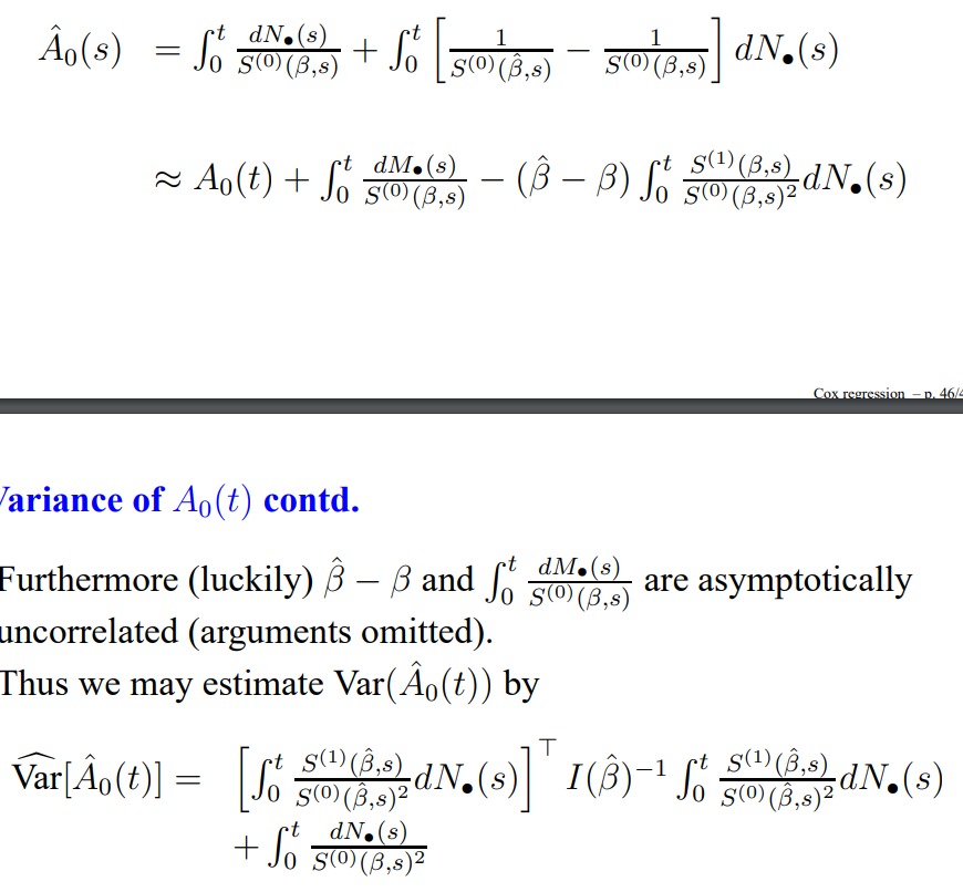
One can see from this that the covariance between \(\hat{\beta}\) and the Breslow estimator is going to be…
cov_breslow_beta <- -var_beta * cumsum(s_1 / s_0 ^ 2) Now we are ready to use the delta method (where \(\Sigma\) is the covariance matrix between the Breslow estimator and \(\hat{\beta}\)):
\[\text{var} \left\lbrace \hat{A}_0 \exp(x\hat{\beta}) \right\rbrace = (\exp(x\hat{\beta}), x\hat{A}_0 \exp(x\hat{\beta}))\hat{\Sigma} (\exp(x\hat{\beta}), x\hat{A}_0 \exp(x\hat{\beta}))^T\]
Applying this to our example:
var_chaz_B <- numeric(length(H_0))
for (i in seq_along(H_0)){

  Sigma_hat_i <- matrix(c(var_breslow[i], cov_breslow_beta[i],
                          cov_breslow_beta[i], var_beta), 2, 2)

  var_chaz_B[i] <- c(exp(beta_hat), H_0[i] * exp(beta_hat)) %*%
                   Sigma_hat_i %*%
                   c(exp(beta_hat), H_0[i] * exp(beta_hat))
}

sqrt(var_chaz_B)
## [1] 0.1313337 0.2049614 0.2853216 0.3685374 0.4799235 0.6046534 0.8159658
## [8] 1.0923455 2.1694201surv_cox$std.err[,2]## [1] 0.1313337 0.2049614 0.2853216 0.3685374 0.4799235 0.6046534 0.8159658
## [8] 1.0923455 2.1694201Step 4 (bonus). Confidence interval for survival curve
I’ll just focus on the lower confidence bounds:
surv_cox$lower## 1 2
## [1,] 0.732485749 0.6831947370
## [2,] 0.577631682 0.5154300933
## [3,] 0.447050313 0.3754471028
## [4,] 0.332545266 0.2655287902
## [5,] 0.234962333 0.1705416091
## [6,] 0.150519749 0.1014505772
## [7,] 0.084192245 0.0458881994
## [8,] 0.033060280 0.0154040543
## [9,] 0.005050267 0.0005498878Having found the standard error for the cumulative hazard, it’s easy to convert this into a confidence interval for the survival curve:
cbind(exp(-(H_0 + sqrt(var_breslow) * qnorm(.975))),
      exp(-(H_0 * exp(beta_hat) + sqrt(var_chaz_B) * qnorm(.975))))
## [,1] [,2]
## [1,] 0.732485749 0.6831947370
## [2,] 0.577631682 0.5154300933
## [3,] 0.447050313 0.3754471028
## [4,] 0.332545266 0.2655287902
## [5,] 0.234962333 0.1705416091
## [6,] 0.150519749 0.1014505772
## [7,] 0.084192245 0.0458881994
## [8,] 0.033060280 0.0154040543
## [9,] 0.005050267 0.0005498878Confidence interval for marginal survival curve
Having established how surfit.coxph calculates standard errors and confidence intervals for a particular fixed covariate \(x\), the next question is: can one produce a confidence interval for the marginal survival curve, standardized over a distribution on \(x\), for example the distribution from the original data set?
I don’t know an “official” answer for this, but based on the above, one option that occurs to me is to simulate from the normal approximation to the joint distribution of \((\hat{A}_0, \hat{\beta})\), then, for each realization, calculate the marginal survival probability, then take quantiles.
We can try it, anyway.
library(mvtnorm)

## set up dummy vector to store results
marginal_mean <- numeric(length(H_0))
marginal_lower <- numeric(length(H_0))
marginal_upper <- numeric(length(H_0))

## function to calculate the mean survival curve
## averaged across the covariates in the original
## data frame.
## Note that the normal approximation to the cumulative
## hazard may stray below 0 (meaning survival above 1),
## so I have to use pmin here:
get_mean_surv <- function(sims){
  mean(pmin(1, exp(-sims[1] * exp(sims[2] * df$x))))
}


## For each time point t_i...
for (i in seq_along(H_0)){

  ## ...extract mean...
  Mu_hat_i <- c(H_0[i], beta_hat)

  ## ...and covariance of (Breslow, beta_hat)
  Sigma_hat_i <- matrix(c(var_breslow[i], cov_breslow_beta[i],
                          cov_breslow_beta[i], var_beta), 2, 2)

  ## simulate from this distribution
  sims_i <- rmvnorm(10000, mean = Mu_hat_i, sigma = Sigma_hat_i)

  ## find the marginal survival curve for each realization
  mean_surv_i <- apply(sims_i, 1, get_mean_surv)

  ## store mean and quantiles to use as estimate and CI
  marginal_mean[i] <- mean(mean_surv_i)
  marginal_lower[i] <- quantile(mean_surv_i, c(0.025))
  marginal_upper[i] <- quantile(mean_surv_i, c(0.975))

}

## Print result for our example
cbind(mean = marginal_mean,
      lower = marginal_lower,
      upper = marginal_upper)
## mean lower upper
## [1,] 0.8880155 0.696913234 1.0000000
## [2,] 0.7972256 0.554475707 1.0000000
## [3,] 0.7049566 0.436028562 1.0000000
## [4,] 0.6157913 0.341393835 1.0000000
## [5,] 0.5244201 0.253445004 1.0000000
## [6,] 0.4343175 0.175397268 1.0000000
## [7,] 0.3425416 0.107482202 1.0000000
## [8,] 0.2483972 0.049395838 1.0000000
## [9,] 0.1469971 0.006160858 0.9667786Obviously, this toy data set is too small to rely on the normal approximations here. But in principle I think this method is reasonable. Of course, it assumes the Cox model is correct.
Dominic Magirr
Medical Statistician
Interested in the design, analysis and interpretation of clinical trials.