Be careful with standard errors in `survival::survfit`
(Mild) panic
In my previous post I looked into how survival::survfit produces standard errors and confidence intervals for a survival curve based on a Cox proportional hazards model. I discovered (I could also have just read it from the documentation) that when you ask for the standard error fit_1$std.err after fit_1 <- survfit(...), it provides you not with the standard error of the estimator of the survival probability, but instead with the standard error of the estimator of the cumulative hazard.
It then occurred to me that I had been using survival::survfit in two of my recent papers. And I had been extracting the standard errors in order to calculate a test statistic for the difference between milestone survival probabilities on the two treatment arms of a clinical trial.
“Oh s***…have I included standard errors for the wrong thing?…are my results wrong?…am I going to have to submit corrections to the articles?”
This motivated me to look more closely again at what survival::survfit is doing. Something I obviously should have done as I was writing the papers!
Kaplan-Meier estimation
My examples just involved Kaplan-Meier estimation and not a Cox model, so I’ll quickly fit a KM for a toy example.
### create a toy data set
df <- data.frame(time = c(3,5,7,12,17,19,25,26,30),
                 event = rep(1,9))

### Kaplan-Meier estimate
library(survival)
fit <- survfit(Surv(time, event) ~ 1, data = df)
fit$std.err
## [1] 0.1178511 0.1781742 0.2357023 0.2981424 0.3726780 0.4714045 0.6236096
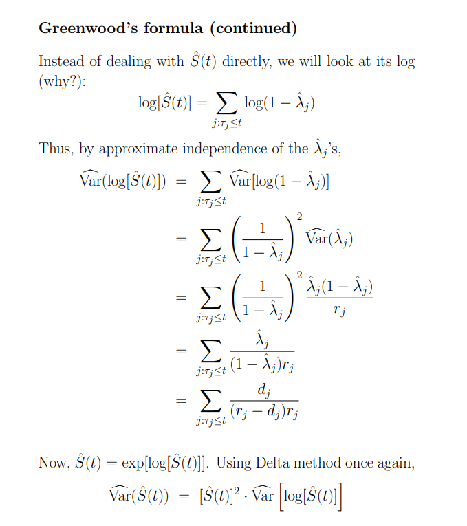
## [8] 0.9428090 InfAs mentioned, this is the standard error for the cumulative hazard. I could have derived it “manually” based on the formulas in slide 22 of this presentation https://mathweb.ucsd.edu/~rxu/math284/slect2.pdf, noting that \(\log(S)=-H\),
n_at_risk <- 9:1
event <- rep(1, 9)
var_H <- cumsum(event / (n_at_risk - event) / n_at_risk)
sqrt(var_H)
## [1] 0.1178511 0.1781742 0.2357023 0.2981424 0.3726780 0.4714045 0.6236096
## [8] 0.9428090 Inf### this matches
fit$std.err## [1] 0.1178511 0.1781742 0.2357023 0.2981424 0.3726780 0.4714045 0.6236096
## [8] 0.9428090 InfWhat happens when you apply summary.survfit?
The summary.survfit method is useful for getting some more detailed information about your model.
summary(fit)## Call: survfit(formula = Surv(time, event) ~ 1, data = df)
##
## time n.risk n.event survival std.err lower 95% CI upper 95% CI
## 3 9 1 0.889 0.105 0.7056 1.000
## 5 8 1 0.778 0.139 0.5485 1.000
## 7 7 1 0.667 0.157 0.4200 1.000
## 12 6 1 0.556 0.166 0.3097 0.997
## 17 5 1 0.444 0.166 0.2141 0.923
## 19 4 1 0.333 0.157 0.1323 0.840
## 25 3 1 0.222 0.139 0.0655 0.754
## 26 2 1 0.111 0.105 0.0175 0.705
## 30 1 1 0.000 NaN NA NANotice here that the std.err looks different to before, and indeed…
summary(fit)$std.err## [1] 0.1047566 0.1385799 0.1571348 0.1656347 0.1656347 0.1571348 0.1385799
## [8] 0.1047566 NaN### is not the same as
fit$std.err## [1] 0.1178511 0.1781742 0.2357023 0.2981424 0.3726780 0.4714045 0.6236096
## [8] 0.9428090 InfIt turns out summary(fit)$std.err is giving the standard error of the estimator of the survival probability. From the formula at the bottom of the slide (printed above), we see that this is just equal to the estimate of the survival probability multiplied by the standard error of the cumulative hazard:
sqrt(var_H) * fit$surv## [1] 0.1047566 0.1385799 0.1571348 0.1656347 0.1656347 0.1571348 0.1385799
## [8] 0.1047566 NaN### this matches
summary(fit)$std.err## [1] 0.1047566 0.1385799 0.1571348 0.1656347 0.1656347 0.1571348 0.1385799
## [8] 0.1047566 NaNFortunately, I’d been using summary(fit)$std.err and not fit$std.err in my code, so I could breathe a sigh of relief.
Confidence intervals
Although it turned out I hadn’t made an error in my papers, I’m still a bit disappointed I didn’t think more carefully about this issue. A standard error for \(S\) suffers from the obvious limitation that \(S\) is restricted to \((0,1)\). A standard error for \(\log(S)\) is probably better, but \(\log(S)\) is still restricted to \((-\infty, 0)\). A standard error for \(\log(-\log(S))\) might be the best option. survfit allows you to use these transformations when constructing confidence intervals.
Confidence intervals for S based on s.e.(S)
### task: can I reproduce confidence intervals?
fit_plain <- survfit(Surv(time, event) ~ 1, data = df, conf.type = "plain")

## reported lower CI for S
fit_plain$lower
## [1] 0.68356980 0.50616616 0.35868804 0.23091758 0.11980647 0.02535471 0.00000000
## [8] 0.00000000 NaN## standard error of cumulative hazard
se_H <- fit_plain$std.err
## standard error of S
se_S <- se_H * fit_plain$surv
## lower CI (forced to be between 0 and 1)
pmax(0, pmin(1, fit_plain$surv - se_S * qnorm(.975)))## [1] 0.68356980 0.50616616 0.35868804 0.23091758 0.11980647 0.02535471 0.00000000
## [8] 0.00000000 NaN## this matches
fit_plain$lower## [1] 0.68356980 0.50616616 0.35868804 0.23091758 0.11980647 0.02535471 0.00000000
## [8] 0.00000000 NaNConfidence intervals for S based on s.e.(log(S))
### task: can I reproduce confidence intervals?
fit_log <- survfit(Surv(time, event) ~ 1, data = df, conf.type = "log")

## reported lower CI for S
fit_log$lower
## [1] 0.70555750 0.54852119 0.42002836 0.30970501 0.21408853 0.13231787 0.06545910
## [8] 0.01750802 NA## standard error of cumulative hazard
se_H <- fit_log$std.err
## standard error of log(S)
se_log_S <- se_H
## lower CI (forced to be less than 1)
pmin(1, exp(log(fit_log$surv) - se_log_S * qnorm(.975)))## [1] 0.70555750 0.54852119 0.42002836 0.30970501 0.21408853 0.13231787 0.06545910
## [8] 0.01750802 0.00000000## this matches
fit_log$lower## [1] 0.70555750 0.54852119 0.42002836 0.30970501 0.21408853 0.13231787 0.06545910
## [8] 0.01750802 NAConfidence intervals for S based on s.e.(log(-log(S)))
### task: can I reproduce confidence intervals?
fit_log_log <- survfit(Surv(time, event) ~ 1, data = df, conf.type = "log-log")

## reported lower CI for S
fit_log_log$lower
## [1] 0.432965090 0.364751231 0.281682242 0.204241776 0.135872478 0.078289473
## [7] 0.033711455 0.006129242 NA## standard error of cumulative hazard
se_H <- fit_log_log$std.err
## standard error of log(-log((S)) [by delta method -- see slide deck]
se_log_log_S <- se_H / log(fit_log_log$surv)
## lower CI
exp(-exp(log(-log(fit_log_log$surv)) - se_log_log_S * qnorm(.975)))## [1] 0.432965090 0.364751231 0.281682242 0.204241776 0.135872478 0.078289473
## [7] 0.033711455 0.006129242 NaN## this matches
fit_log_log$lower## [1] 0.432965090 0.364751231 0.281682242 0.204241776 0.135872478 0.078289473
## [7] 0.033711455 0.006129242 NADominic Magirr
Medical Statistician
Interested in the design, analysis and interpretation of clinical trials.