Conditional and unconditional treatment effects in RCTs
Small simulation study
Quick function to simulate data from an RCT with equal allocation to treatments 0 and 1, a single covariate, and a binary endpoint:
sim_data <- function(n){

  z <- rep(0:1, each = n / 2) ## trt assignment

  x <- rnorm(n) ## covariate

  eta <- -1 +  2 * x  - log(0.55) * z ## linear predictor

  pi <- exp(eta) / (1 + exp(eta)) ## prob(outcome = 1)

  y <- rbinom(n, 1, pi) ## outcome

  data.frame(z, x, y)
}
The data generating mechansim is a logistic model (but also see later). I’ll draw it
x <- seq(-2, 2, length.out = 100)
plot(x, plogis(-1 + 2 * x), ylim = c(0,1), type = "l", ylab = "P(Y=1)")
points(x, plogis(-1 +  2 * x - log(0.55)), col = 2, type = "l")
legend("topleft", c("Z=0", "Z=1"), lty = c(1,1), col = c(1,2))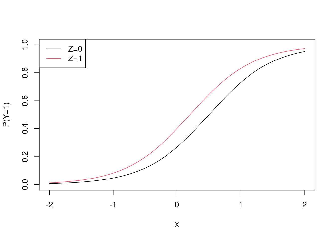
Now I’ll write a function to give me:
- Direct adjustment via logistic regression including terms for treatment and the covariate. Giving conditional log-odds ratio.
- Standardization of (1) to give the unconditional log-odds ratio (using the
stdRegpackage). - Unadjusted analysis: logistic regression with just a term for treatment. Giving unconditional log-odds ratio.
library("stdReg")
######################################
sim_one_trial_with_analysis <- function(n){

  ### simulate data
  dat <- sim_data(n)

  ### fit a direct adjustment model...
  fit_dir_adj <- glm(y ~ x + z, family = "binomial", data = dat)

  ### ...extract point estimate and z statistic
  dir_adj_est <- summary(fit_dir_adj)$coef["z", "Estimate"]
  dir_adj_z   <- summary(fit_dir_adj)$coef["z", "z value"]

  ### apply standardization / g-formula...
  std_fit <- stdReg::stdGlm(fit_dir_adj, data = dat, X = "z")
  sum_std_fit <- summary(std_fit,
                         transform = "logit",
                         contrast = "difference",
                         reference = 0)

  ### ...extract point estimate and z statistic
  g_est <- sum_std_fit$est.table["1", "Estimate"]
  g_z   <- g_est / sum_std_fit$est.table["1", "Std. Error"]


  ### fit unadjusted model...
  fit_unadj <- glm(y ~  z, family = "binomial", data = dat)


  ### ...extract point estimate and z statistic
  unadj_est <- summary(fit_unadj)$coef["z", "Estimate"]
  unadj_z   <- summary(fit_unadj)$coef["z", "z value"]


  data.frame(dir_adj_est = dir_adj_est,
             dir_adj_z = dir_adj_z,
             g_est = g_est,
             g_z = g_z,
             unadj_est = unadj_est,
             unadj_z = unadj_z)


}
I’ll use this to simulate 1000 trials each with sample size 300…
res <- purrr::map_df(rep(300, 1000), sim_one_trial_with_analysis)and plot the results, firstly in terms of the point estimates…
par(mfrow = c(1,2))
plot(res$g_est, res$unadj_est,
     xlim = c(-0.5, 2),
     ylim = c(-0.5, 2),
     xlab = "log(OR) 'standardization'",
     ylab = "log(OR) 'unadjusted'")
abline(a=0,b = 1,col = 2,lwd = 3)
plot(res$g_est, res$dir_adj_est,
     xlim = c(-0.5, 2),
     ylim = c(-0.5, 2),
     xlab = "log(OR) 'standardization'",
     ylab = "log(OR) 'direct adjusted'")
abline(a=0,b = 1,col = 2,lwd = 3)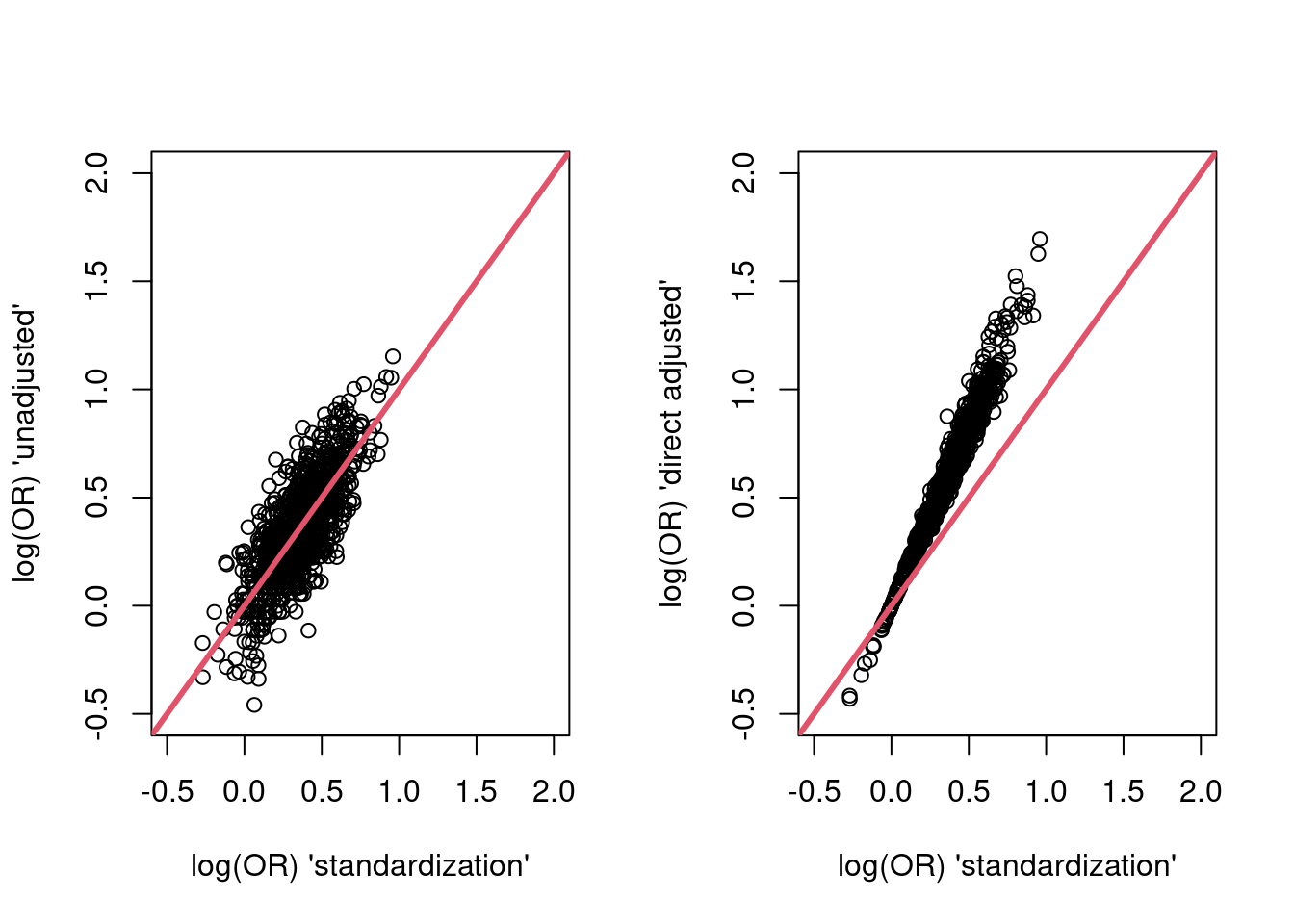
The standardized and unadjusted estimates do not appear systematically different. The directly adjusted point estimates are systematically larger (because they are estimates of a different parameter - the condidional log-odds ratio).
Now the standardized Z-statistics…
par(mfrow = c(1,2))
plot(res$g_z, res$unadj_z,
     xlab = "Z 'standardization'",
     ylab = "Z 'unadjusted'")
abline(a=0,b = 1,col = 2,lwd = 3)
abline(h = 2.33, col = 2, lty = 2)
abline(v = 2.33, col = 2, lty = 2)

plot(res$g_z, res$dir_adj_z,
     xlab = "Z 'standardization'",
     ylab = "Z 'direct adjusted'")
abline(a=0,b = 1,col = 2,lwd = 3)
abline(h = 2.33, col = 2, lty = 2)
abline(v = 2.33, col = 2, lty = 2)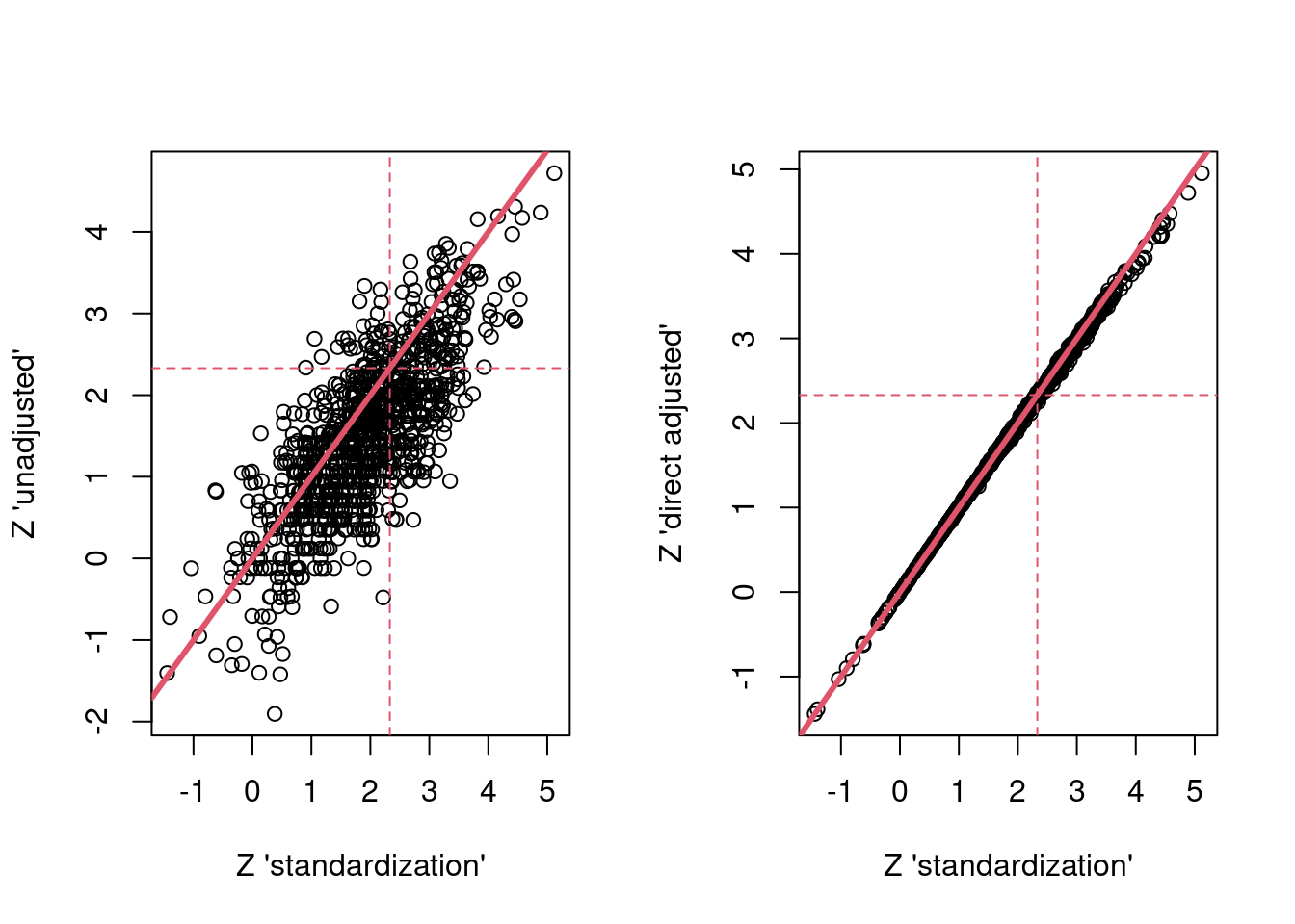
Appendix: misspecified model
I’ll repeat the exercise for a misspecified model example. Here I’ll draw it the data generating mechanism…
x <- seq(-2, 2, length.out = 100)
plot(x, exp(-exp(2 -  2 * x)), ylim = c(0,1), type = "l", ylab = "P(Y=1)")
points(x, exp(-exp(2 -  2 * x  + log(0.4) * x)), col = 2, type = "l")
legend("topleft", c("Z=0", "Z=1"), lty = c(1,1), col = c(1,2))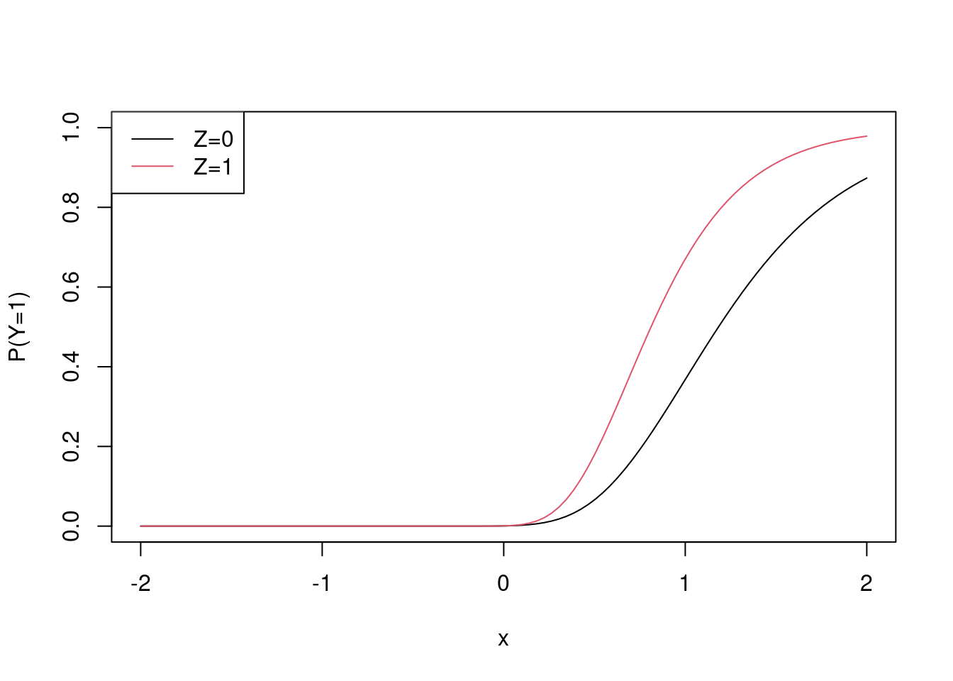
…and here are the results showing similar things…
sim_data <- function(n){

  z <- rep(0:1, each = n / 2)

  x <- rnorm(n)

  eta <- 2 -  2 * x  + log(0.4) * z * x

  pi <- exp(-exp(eta))

  y <- rbinom(n, 1, pi)

  data.frame(z, x, y)
}
res <- purrr::map_df(rep(300, 1000), sim_one_trial_with_analysis)## Warning: glm.fit: fitted probabilities numerically 0 or 1 occurred
## Warning: glm.fit: fitted probabilities numerically 0 or 1 occurredpar(mfrow = c(1,2))
plot(res$g_est, res$unadj_est,
xlim = c(-0.5, 2),
ylim = c(-0.5, 2),
xlab = "log(OR) 'standardization'",
ylab = "log(OR) 'unadjusted'")
abline(a=0,b = 1,col = 2,lwd = 3)
plot(res$g_est, res$dir_adj_est,
xlim = c(-0.5, 2),
ylim = c(-0.5, 2),
xlab = "log(OR) 'standardization'",
ylab = "log(OR) 'direct adjusted'")
abline(a=0,b = 1,col = 2,lwd = 3)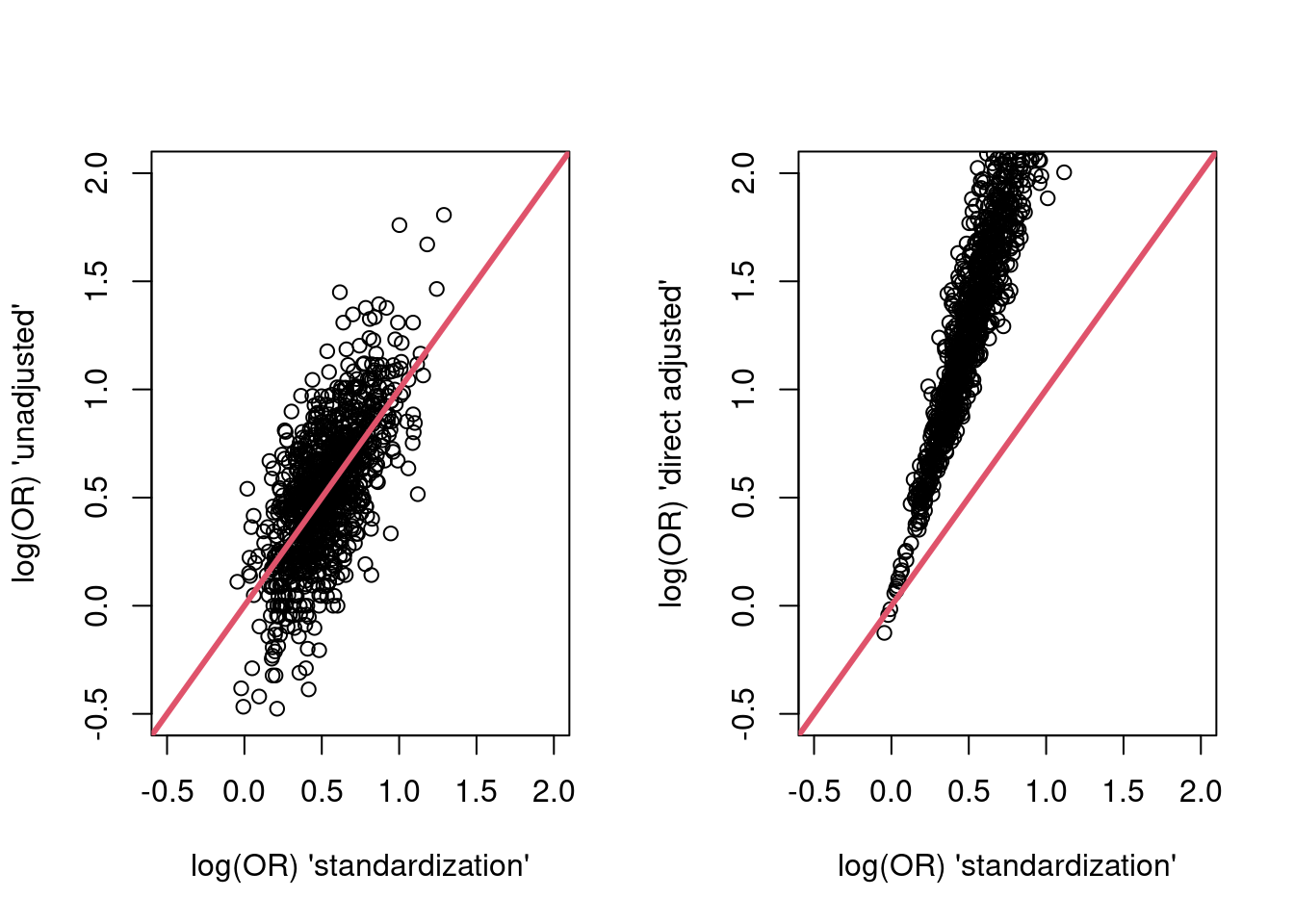
par(mfrow = c(1,2))
plot(res$g_z, res$unadj_z,
     xlab = "Z 'standardization'",
     ylab = "Z 'unadjusted'")
abline(a=0,b = 1,col = 2,lwd = 3)
abline(h = 2.33, col = 2, lty = 2)
abline(v = 2.33, col = 2, lty = 2)


plot(res$g_z, res$dir_adj_z,
     xlab = "Z 'standardization'",
     ylab = "Z 'direct adjusted'")
abline(a=0,b = 1,col = 2,lwd = 3)
abline(h = 2.33, col = 2, lty = 2)
abline(v = 2.33, col = 2, lty = 2)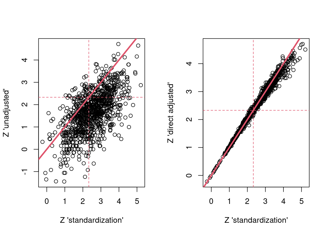
Dominic Magirr
Medical Statistician
Interested in the design, analysis and interpretation of clinical trials.