{nphRCT} on CRAN
I’m delighted that our new R package {nphRCT} is available on CRAN. Special thanks to Isobel Barrot. Her R skills have made this possible. Thanks also to Carl-Fredrik Burman and José Jiménez, my collaborators on this topic over the past few years.
library(dplyr)
library(ggplot2)
library(survival)
#devtools::install_github("https://github.com/cran/nphRCT.git")
library(nphRCT)
The idea for the package was to make it easy to perform a weighted log-rank test, and in particular the modestly-weighted logrank test, in the context of an Randomized Controlled Trial (RCT) where one expects a delayed separation of survival curves.
Example data set
A dataset I often use as an example in this context is the POPLAR trial data.
Let’s find the data from the web, and plot the Kaplan-Meier curves…
template <- tempfile(fileext = ".xlsx")

httr::GET(url = "https://static-content.springer.com/esm/art%3A10.1038%2Fs41591-018-0134-3/MediaObjects/41591_2018_134_MOESM3_ESM.xlsx",
          httr::write_disk(template))
dat <- readxl::read_excel(template,sheet = 2) %>%
select(PtID, ECOGGR, OS, OS.CNSR, TRT01P) %>%
mutate(event = -1 * (OS.CNSR - 1),
time = OS,
arm = ifelse(TRT01P == "Docetaxel", "control", "experimental")) %>%
select(time, event, arm) %>%
as.data.frame()
km <- survfit(Surv(time, event) ~ arm, data = dat)survminer::ggsurvplot(km,
data = dat,
risk.table = TRUE,
break.x.by = 6,
legend.title = "",
xlab = "Time (months)",
ylab = "Overall survival",
risk.table.fontsize = 4,
legend = c(0.8,0.8))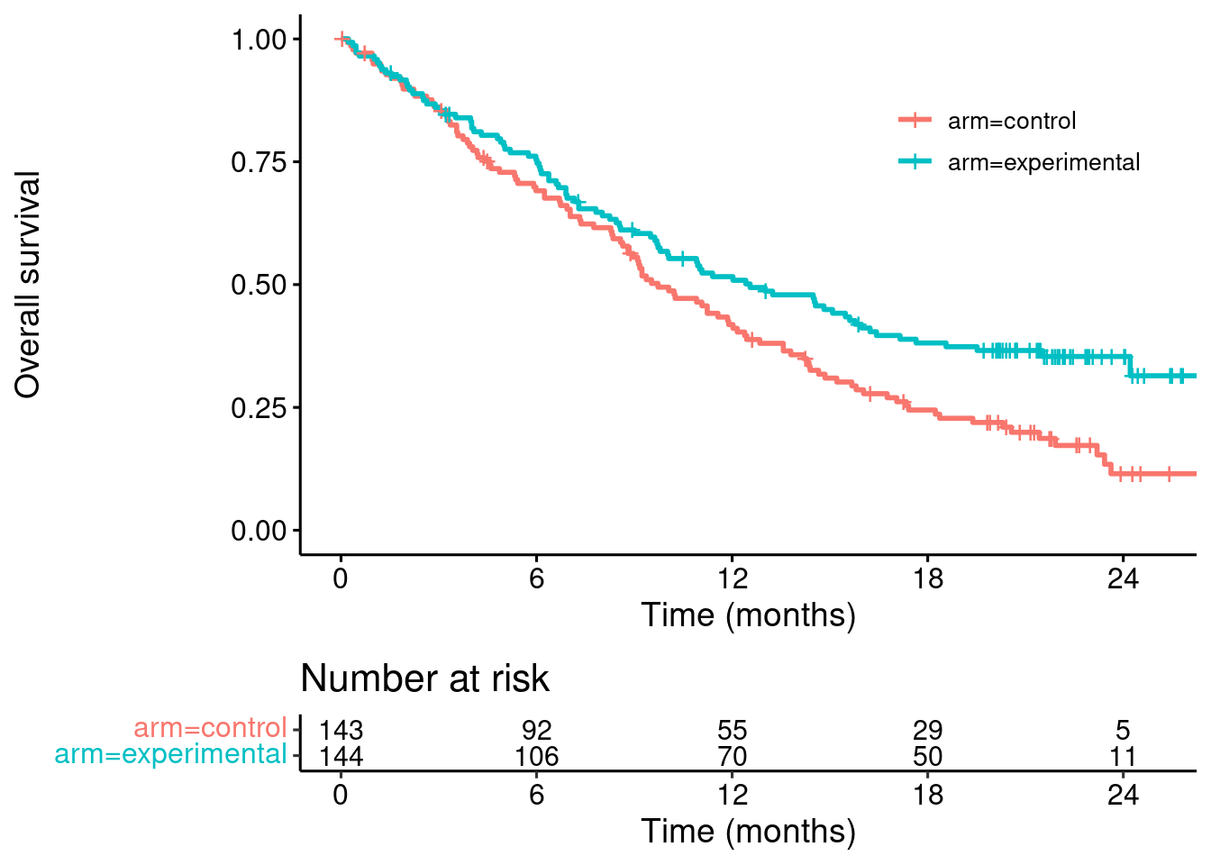
At-risk table
The at-risk table (per arm) may be a good place to start. If we want, we can look at this via find_at_risk. The syntax should be familiar from the {survival} package.
at_risk <- nphRCT::find_at_risk(Surv(time, event) ~ arm,
                                data = dat,
                                include_cens = FALSE)

head(at_risk)
## t_j n_event_control n_event_experimental n_event n_risk_control
## 1 0.1971253 1 0 1 138
## 2 0.2299795 0 1 1 137
## 3 0.2956879 1 0 1 137
## 4 0.3613963 1 1 2 136
## 5 0.4599589 1 2 3 135
## 6 0.5585216 0 1 1 134
## n_risk_experimental n_risk
## 1 144 282
## 2 144 281
## 3 143 280
## 4 143 279
## 5 142 277
## 6 140 274The weighted log-rank test statistic is
\[ U^W = \sum_{j=1}^k w_j \left\lbrace \text{n_event_control}(t_{j}) - \text{n_event}(t_{j}) \times \frac{\text{n_risk_control}(t_{j})}{\text{n_risk}(t_{j})}\right\rbrace \]
Weights
Modestly-weighted
The modestly weighted log-rank test uses weights \(w_j = 1 / \max\{\hat{S}(t_j-), s^*\}\), where \(\hat{S}(t_j-)\) is the Kaplan-Meier estimate at \(t_j-\) (just prior to event time \(t_j\)) based on the pooled (both arms) data, and \(s^* \in (0,1]\) is pre-specified. For example, taking \(s^*=0.5\)…
weights_mw_s <- nphRCT::find_weights(Surv(time, event) ~ arm,
                                     data = dat,
                                     method = "mw",
                                     s_star = 0.5)


plot(at_risk$t_j, weights_mw_s, ylim = c(0,2),
     xlab = "Event time",
     ylab = "Weight",
     main = "Modestly weighted, s*=0.5")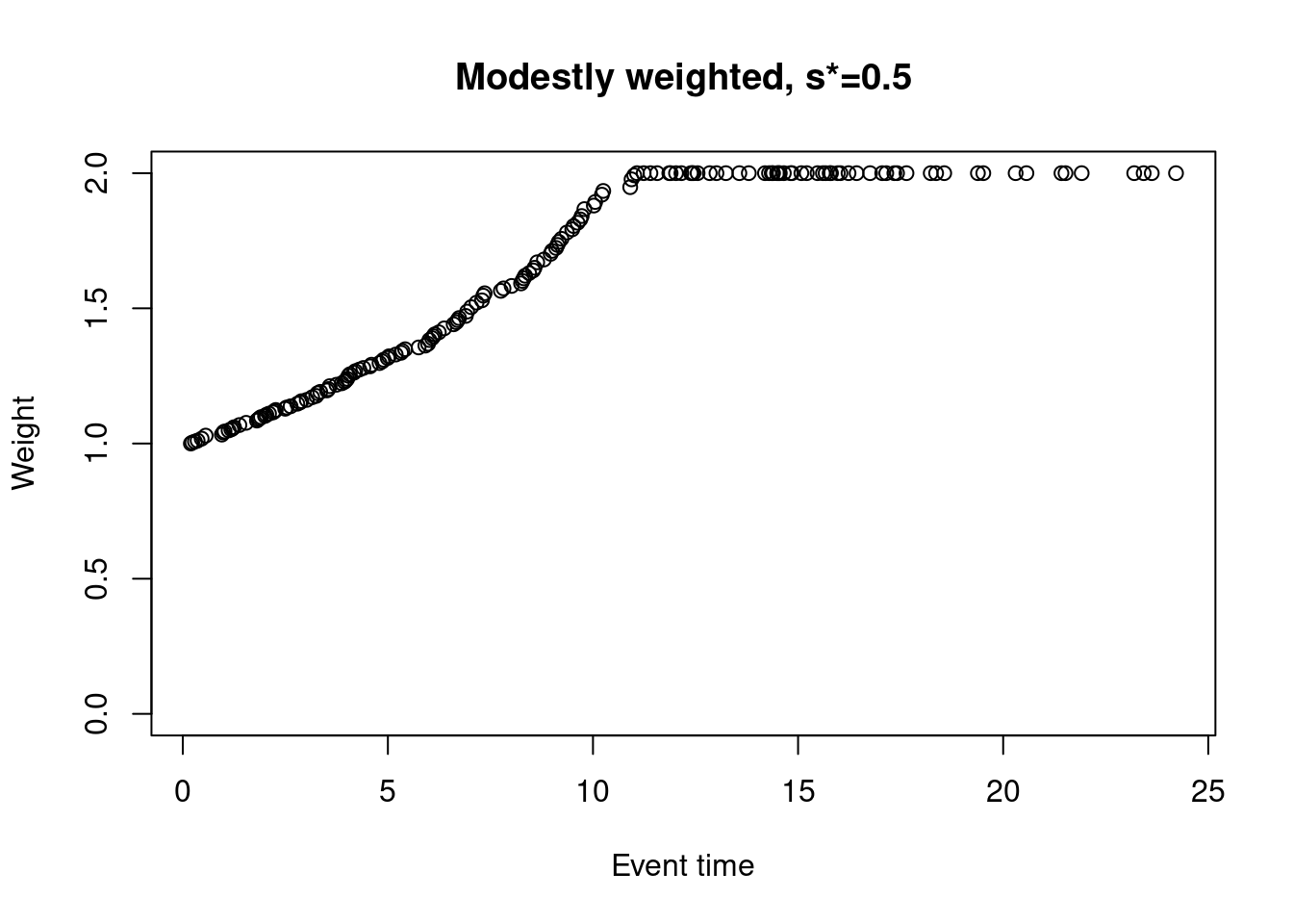
In this case, the weight for the first event time is 1, and weights are increasing but capped at 2 at the time the KM curve drops to 0.5 (at around 12 months).
Alternatively, one could choose \(w_j = 1 / \max\{\hat{S}(t_j-), \hat{S}(t^*)\}\), where \(t^*\) is a pre-specified timepoint beyond which the weights no longer increase. The weights are then capped at \(1 / \hat{S}(t^*)\). For example, taking \(t^* = 6\),
weights_mw_t <- nphRCT::find_weights(Surv(time, event) ~ arm,
                                     data = dat,
                                     method = "mw",
                                     t_star = 6)


plot(at_risk$t_j, weights_mw_t, ylim = c(0,2),
     xlab = "Event time",
     ylab = "Weight",
     main = "Modestly weighted, t*=6")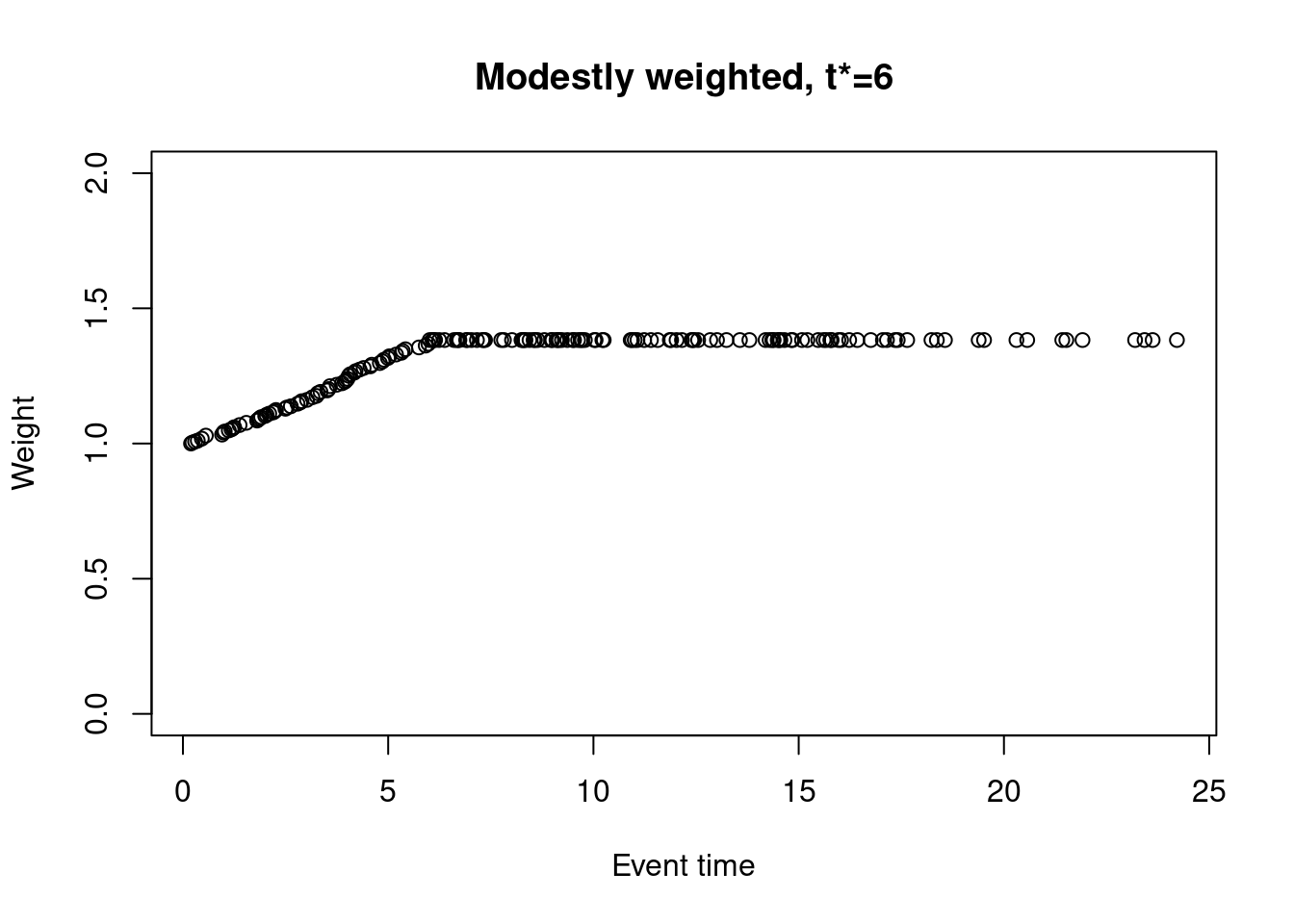
Special case: \(s^*=1\) (or \(t^*=0\))
The special case \(s^*=1\) (or \(t^*=0\)) is the same as the standard log-rank test.
Fleming-Harrington \((\rho, \gamma)\) test
The Fleming-Harrington \((\rho, \gamma)\) weights are \(\hat{S}(t_j-)^{\rho}\{1 - \hat{S}(t_j-) \}^{\gamma}\). Often, in delayed effect scenarios, \(\rho=0\) and \(\gamma=1\) is chosen.
weights_fh_0_1 <- nphRCT::find_weights(Surv(time, event) ~ arm,
data = dat,
method = "fh",
rho = 0,
gamma = 1)
plot(at_risk$t_j, weights_fh_0_1, ylim = c(0,1),
xlab = "Event time",
ylab = "Weight",
main = "Fleming-Harrington (0,1)")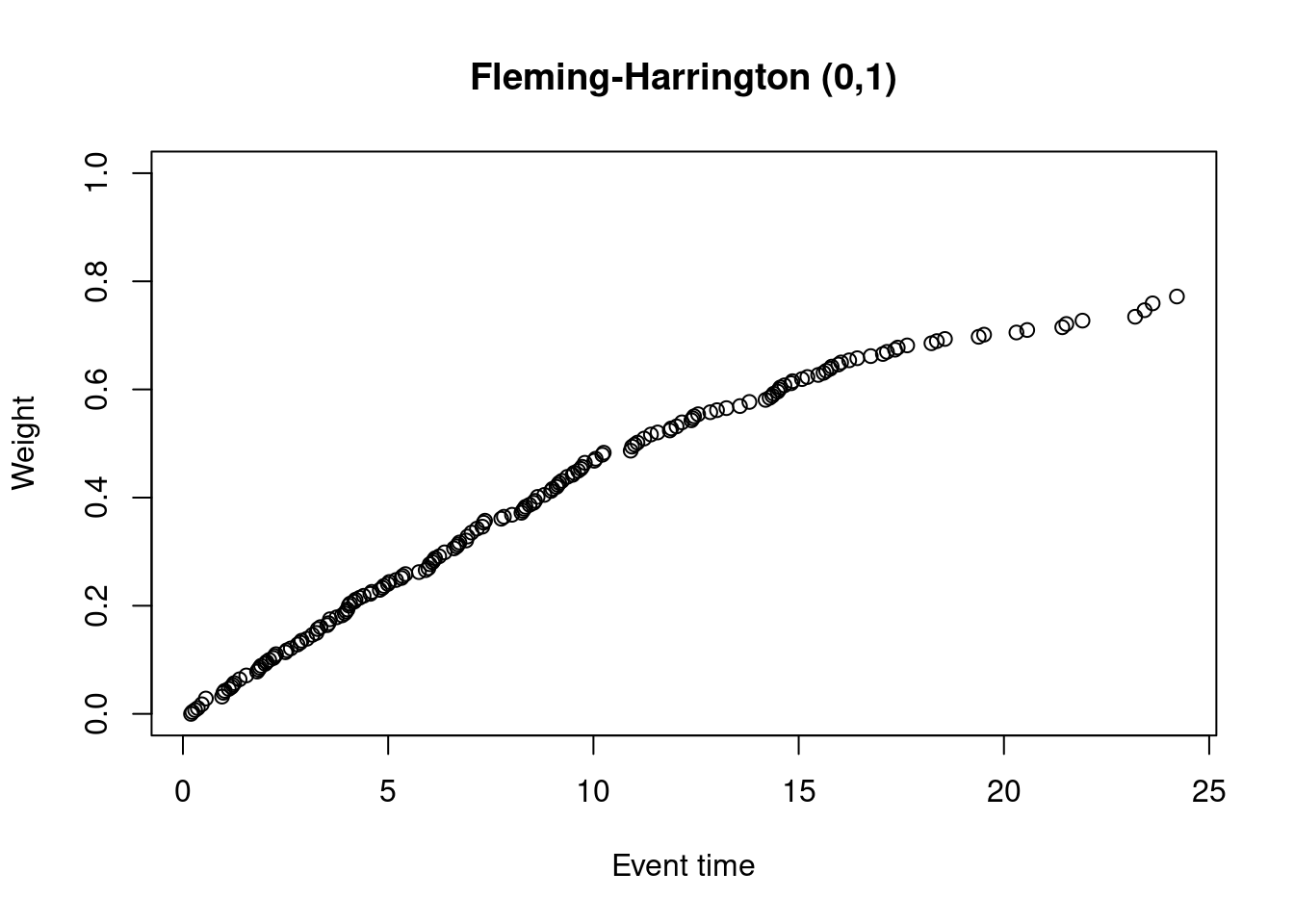 The main difference between F-H(0,1) weights and the modest weights is that the F-H(0,1) weights start at zero. The early events are therefore much more heavily down-weighted compared to the modest test.
Special case: \(\rho = \gamma = 0\)
The special case \(\rho = \gamma = 0\) is the same as the standard log-rank test.
Performing the weighted log-rank test
To perform the weighed log-rank test use the wlrt function.
# Modestly-weighted (t*=6)
nphRCT::wlrt(Surv(time, event) ~ arm,
             data = dat,
             method = "mw",
             t_star = 6)
## u v_u z trt_group
## 1 -26.11708 83.62023 -2.856071 experimental# Standard log-rank test (t*=0)
nphRCT::wlrt(Surv(time, event) ~ arm,
data = dat,
method = "mw",
t_star = 0)## u v_u z trt_group
## 1 -19.42566 49.15217 -2.770796 experimental# Fleming-Harrington (0,1)
nphRCT::wlrt(Surv(time, event) ~ arm,
data = dat,
method = "fh",
rho = 0,
gamma = 1)## u v_u z trt_group
## 1 -9.942946 8.522577 -3.405882 experimentalVisualization of test statistic: difference in mean score
It’s possible to visualize a weighted log-rank test as a difference in mean “score” on the two treatment arms, where the scores are a transformation of the 2-dimensional outcomes (time, event status) to the real line. This is explained in more detail here.
We’ll try it now for our examples. In these plots, each dot corresponds to a patient in the trial. On the x-axis is their time-to-event/censoring, and on the y-axis is their score. For the log-rank test, we see two almost parallel lines, with the top line corresponding to the observed events, and the bottom line corresponding to censored observations. So someone who dies at month 1 gets a score close to 1 (the worst score), and someone who is censored at month 24 gets a score close to -1 (the best score). Note that the scaling is arbitrary. The dashed horizontal lines represent the mean score on the two treatment arms. The difference between these to lines is the log-rank test statistic (a re-scaled version of it).
# Standard log-rank test (t*=0)
nphRCT::find_scores(Surv(time, event) ~ arm,
             data = dat,
             method = "mw",
             t_star = 0) %>% plot()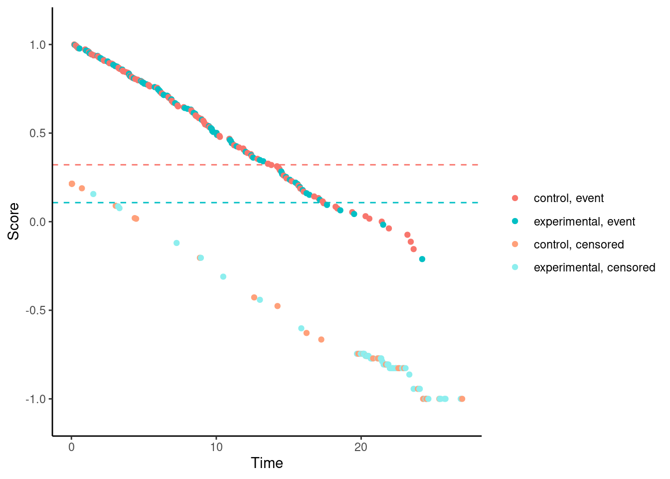
For the modestly-weighted test, the scores (for observed events) are essentially fixed at 1 until time \(t^*\). This is by design.
# Modestly-weighted (t*=6)
nphRCT::find_scores(Surv(time, event) ~ arm,
             data = dat,
             method = "mw",
             t_star = 6) %>% plot()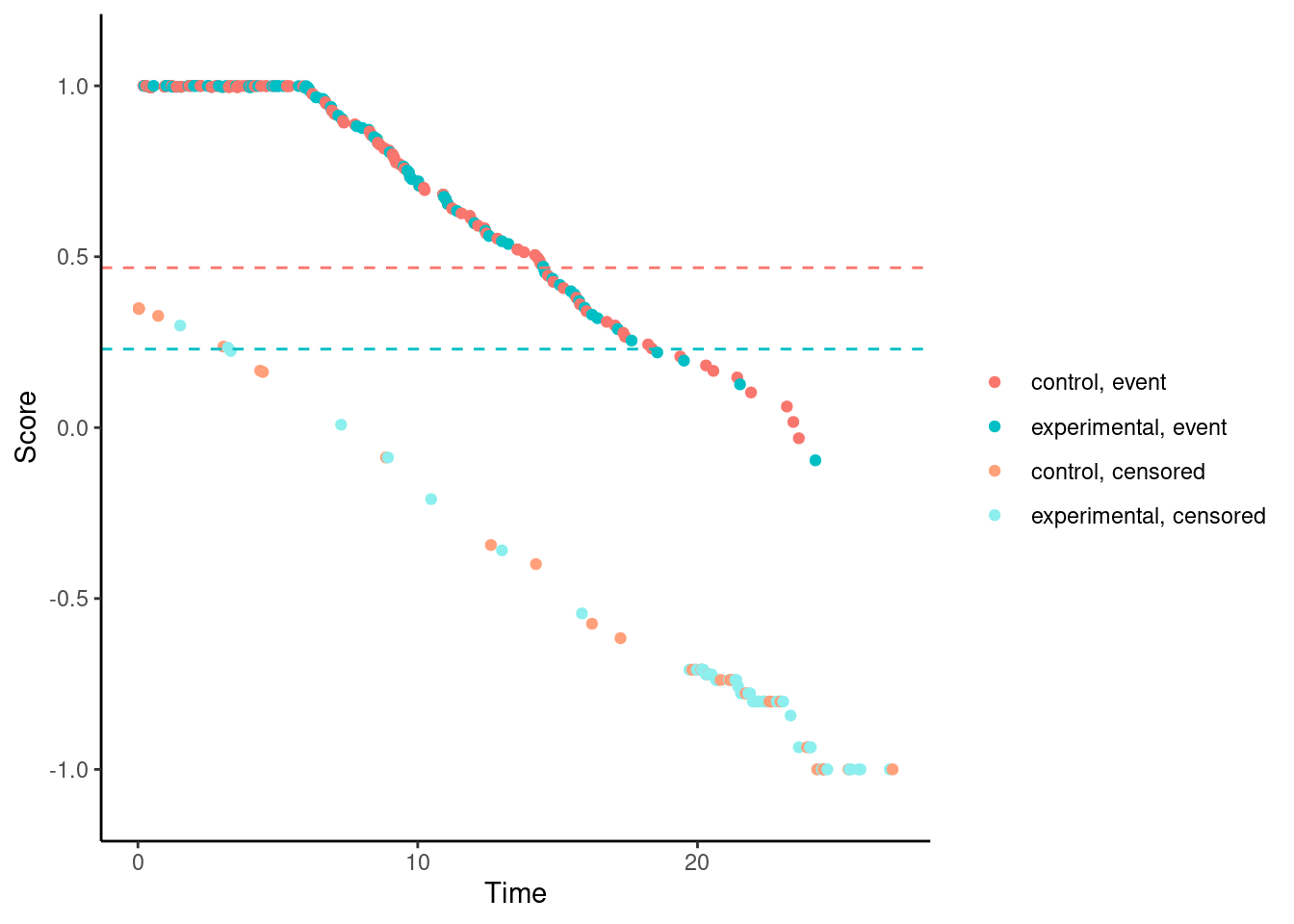
In contrast, for the Fleming-Harrington-(0,1) test, the scores (for observed events) are increasing with time for early follow-up times. So someone who dies at month 1 gets a lower (better) score than someone who dies at month 12. Basically, one has downweighted the early events to such an extent that the test actually “rewards” the experimental treatment for causing early harm.
# Fleming-Harrington (0,1)
nphRCT::find_scores(Surv(time, event) ~ arm,
             data = dat,
             method = "fh",
             rho = 0,
             gamma = 1) %>% plot()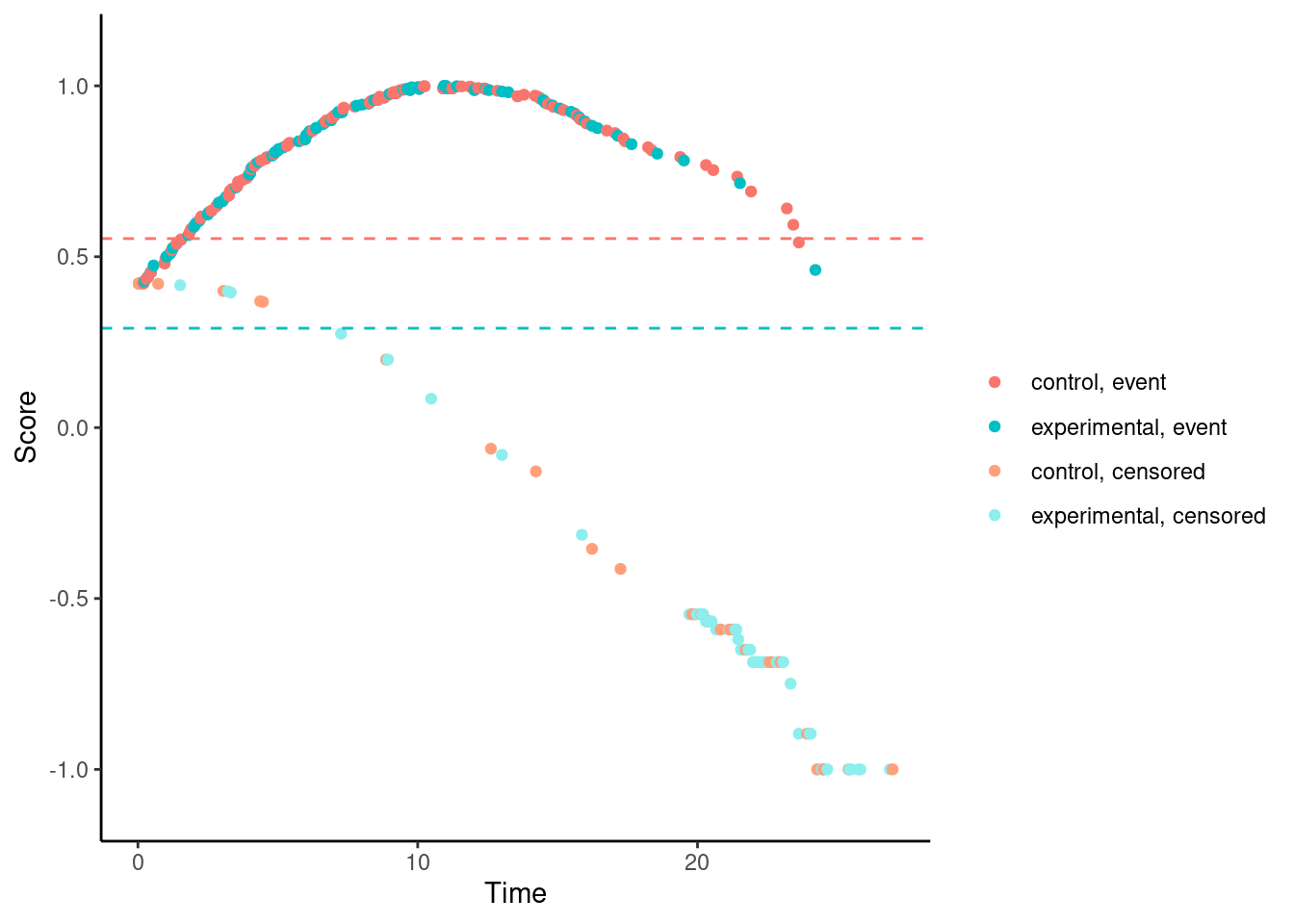
Other versions of Fleming-Harrington test e.g., (1,1), (0,0.5), (0.5,0.5), etc. suffer from the same problem.
# Fleming-Harrington (1,1)
nphRCT::find_scores(Surv(time, event) ~ arm,
             data = dat,
             method = "fh",
             rho = 1,
             gamma = 1) %>% plot()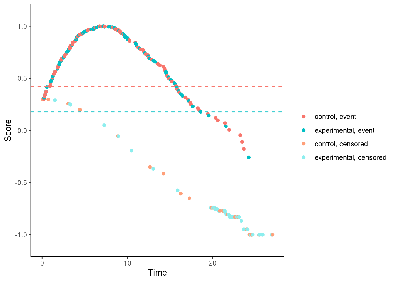
# Fleming-Harrington (0,0.5)
nphRCT::find_scores(Surv(time, event) ~ arm,
             data = dat,
             method = "fh",
             rho = 0,
             gamma = 0.5) %>% plot()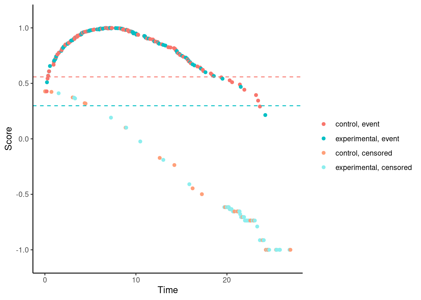
# Fleming-Harrington (0.5,0.5)
nphRCT::find_scores(Surv(time, event) ~ arm,
             data = dat,
             method = "fh",
             rho = 0.5,
             gamma = 0.5) %>% plot()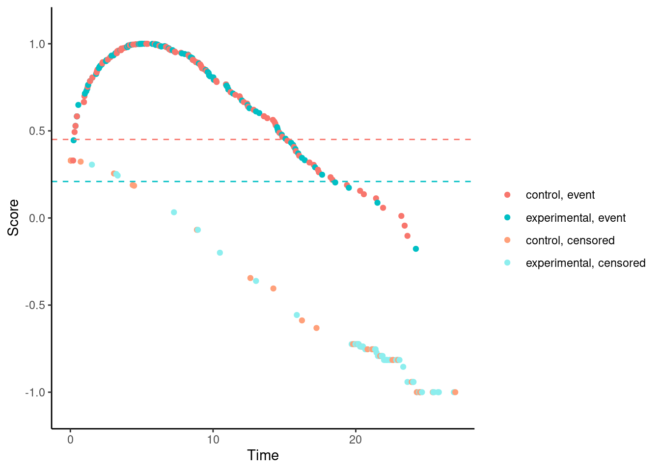
Dominic Magirr
Medical Statistician
Interested in the design, analysis and interpretation of clinical trials.