Adjusting for covariates under non-proportional hazards
I’ve written a lot recently about non-proportional hazards in immuno-oncology. One aspect that I have unfortunately overlooked is covariate adjustment. Perhaps this is because it’s so easy to work with extracted data from published Kaplan-Meier plots, where the covariate data is not available. But we know from theoretical and empirical work that covariate adjustment can lead to big increases in power, and perhaps this is equally important or even more important than the power gains from using a weighted log-rank test to match the anticipated non-proportional hazards. To investigate this, we would need access to immuno-oncology RCT data. In general this is not so easy, but fortunately there’s this article containing clinical data from two RCTs (OAK and POPLAR) comparing a checkpoint inhibitor (atezolizumab) versus chemotherapy.
Gandara, D.R., Paul, S.M., Kowanetz, M. et al. Blood-based tumor mutational burden as a predictor of clinical benefit in non-small-cell lung cancer patients treated with atezolizumab. Nat Med 24, 1441–1448 (2018). https://doi.org/10.1038/s41591-018-0134-3
A number of covariates are provided but I will focus on baseline ECOG grade, which is a performance status indicator – a “0” means fully active; a “1” means restricted in physically strenuous activity. Generally, you would expect patients with lower ECOG status to have longer survival.
Let’s have a look at the OAK data first…
library(tidyverse)
library(survival)

## Here I'm loading my library locally...
devtools::load_all("~/swlrt/")

## ...but can also get it from github
#devtools::install_github("dominicmagirr/swlrt")

## read in the clinical data from the OAK study
## create a new column OS.EVENT which is the opposite
## of OS.CNSR

dat_oak <- readxl::read_excel("41591_2018_134_MOESM3_ESM.xlsx",
                              sheet = 3) %>%
  select(PtID, ECOGGR, OS, OS.CNSR, TRT01P) %>%
  mutate(OS.EVENT = -1 * (OS.CNSR - 1))

## take a look at first few rows
head(dat_oak)
## # A tibble: 6 x 6
## PtID ECOGGR OS OS.CNSR TRT01P OS.EVENT
## <dbl> <dbl> <dbl> <dbl> <chr> <dbl>
## 1 318 1 5.19 0 Docetaxel 1
## 2 1088 0 4.83 0 Docetaxel 1
## 3 345 1 1.94 0 Docetaxel 1
## 4 588 0 24.6 1 Docetaxel 0
## 5 306 1 5.98 0 MPDL3280A 1
## 6 718 1 19.2 1 Docetaxel 0It’s standard fare for surival analysis. Let’s first make a Kaplan-Meier plot and fit a Cox model based only on treatment…
km_oak <- survfit(Surv(OS, OS.EVENT) ~ TRT01P,
                  data = dat_oak)

survminer::ggsurvplot(km_oak,
                      data = dat_oak,
                      risk.table = TRUE,
                      break.x.by = 6,
                      legend.title = "",
                      xlab = "Time (months)",
                      ylab = "Overall survival",
                      risk.table.fontsize = 4,
                      legend = c(0.8,0.8))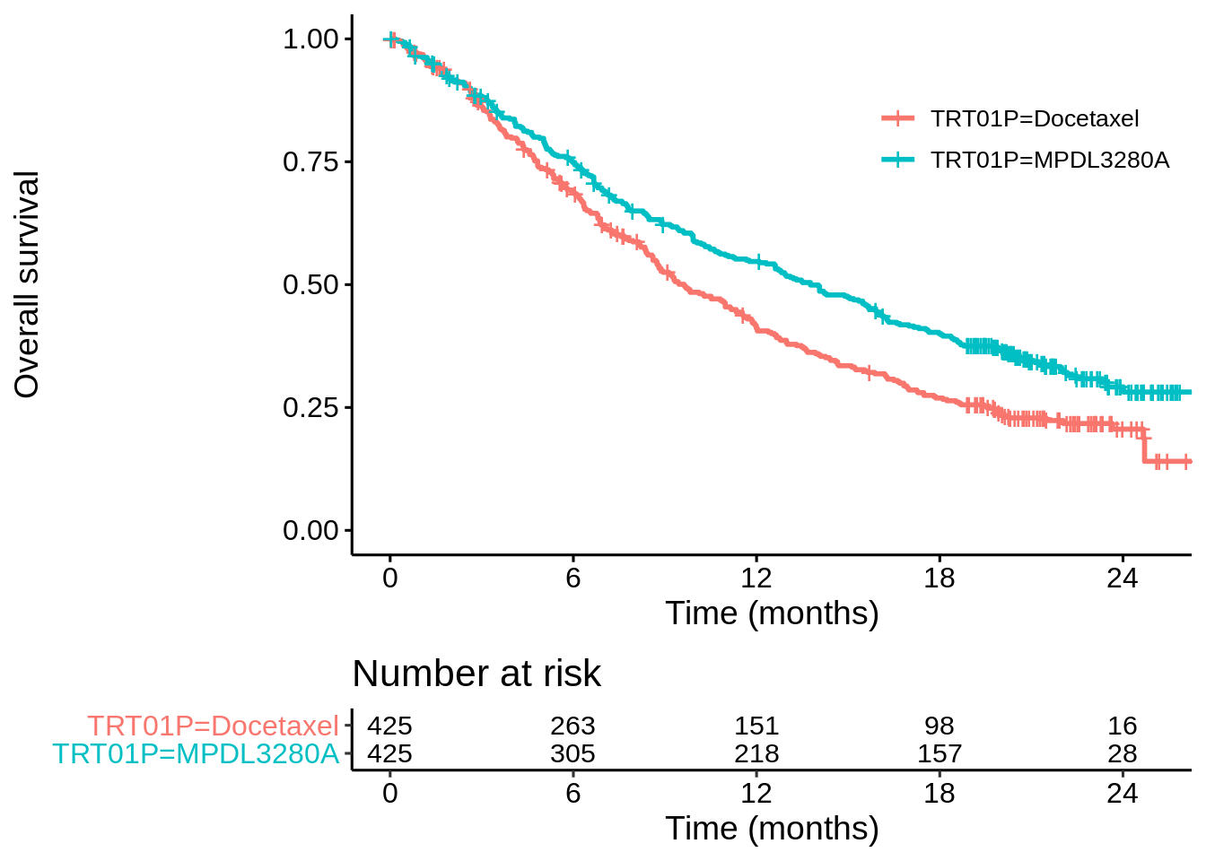
coxph(Surv(OS, OS.EVENT) ~ TRT01P, data = dat_oak)## Call:
## coxph(formula = Surv(OS, OS.EVENT) ~ TRT01P, data = dat_oak)
##
## coef exp(coef) se(coef) z p
## TRT01PMPDL3280A -0.31667 0.72857 0.08418 -3.762 0.000169
##
## Likelihood ratio test=14.16 on 1 df, p=0.0001677
## n= 850, number of events= 569The z-value is -3.762 (lower is better). This should be very similar to the z-value of the log-rank test. Let’s check using a function I’ve written for my own R package swlrt.
swlrt::wlrt(df = dat_oak,
            trt_colname = "TRT01P",
            time_colname = "OS",
            event_colname = "OS.EVENT",
            wlr = "lr")
## u v_u z o_minus_e_trt
## 1 -44.59584 139.4881 -3.775946 MPDL3280AHad the non-proportional hazards been anticipated, a weighted log-rank test could have been pre-specified, for example a modestly-weighted log-rank test with \(t^* = 12\)…
swlrt::wlrt(df = dat_oak,
            trt_colname = "TRT01P",
            time_colname = "OS",
            event_colname = "OS.EVENT",
            wlr = "mw",
            t_star = 12)
## u v_u z o_minus_e_trt
## 1 -74.88024 370.4699 -3.890368 MPDL3280AThis would have had a lower z-value (-3.89), as you’d expect given the slightly delayed effect,
But what about an adjusted analysis?
Let’s look at a Cox model including ECOG grade as a covariate…
coxph(Surv(OS, OS.EVENT) ~ TRT01P + ECOGGR, data = dat_oak)## Call:
## coxph(formula = Surv(OS, OS.EVENT) ~ TRT01P + ECOGGR, data = dat_oak)
##
## coef exp(coef) se(coef) z p
## TRT01PMPDL3280A -0.35234 0.70304 0.08445 -4.172 3.02e-05
## ECOGGR 0.63227 1.88187 0.09072 6.970 3.18e-12
##
## Likelihood ratio test=65.79 on 2 df, p=5.163e-15
## n= 850, number of events= 569Now the z-value is -4.172. So in this example, remembering to adjust for a prognostic covariate appears more important than dealing with the nph issue.
Can’t we do both?
Yes, it’s possible to do the modestly-weighted log-rank test, stratified by ECOG grade:
swlrt::swlrt(df = dat_oak,
             trt_colname = "TRT01P",
             time_colname = "OS",
             event_colname = "OS.EVENT",
             strat_colname = "ECOGGR",
             wlr = "mw",
             t_star = 12)
## $by_strata
## u v_u z o_minus_e_trt
## ECOGGR0 -15.46822 87.47411 -1.653867 MPDL3280A
## ECOGGR1 -71.10216 307.90543 -4.052044 MPDL3280A
##
## $z
## [1] -4.353737Now the z-value is lower still (-4.35), which seems like the best of both worlds.
Will covariate adjustment always improve the z-value?
No. Let’s go through exactly the same steps for the POPLAR study.
## read in the clinical data from the POPLAR study
## create a new column OS.EVENT which is the opposite
## of OS.CNSR
dat_poplar <- readxl::read_excel("41591_2018_134_MOESM3_ESM.xlsx",
                              sheet = 2) %>%
  select(PtID, ECOGGR, OS, OS.CNSR, TRT01P) %>%
  mutate(OS.EVENT = -1 * (OS.CNSR - 1))


km_poplar <- survfit(Surv(OS, OS.EVENT) ~ TRT01P,
                  data = dat_poplar)

survminer::ggsurvplot(km_poplar,
                      data = dat_poplar,
                      risk.table = TRUE,
                      break.x.by = 6,
                      legend.title = "",
                      xlab = "Time (months)",
                      ylab = "Overall survival",
                      risk.table.fontsize = 4,
                      legend = c(0.8,0.8))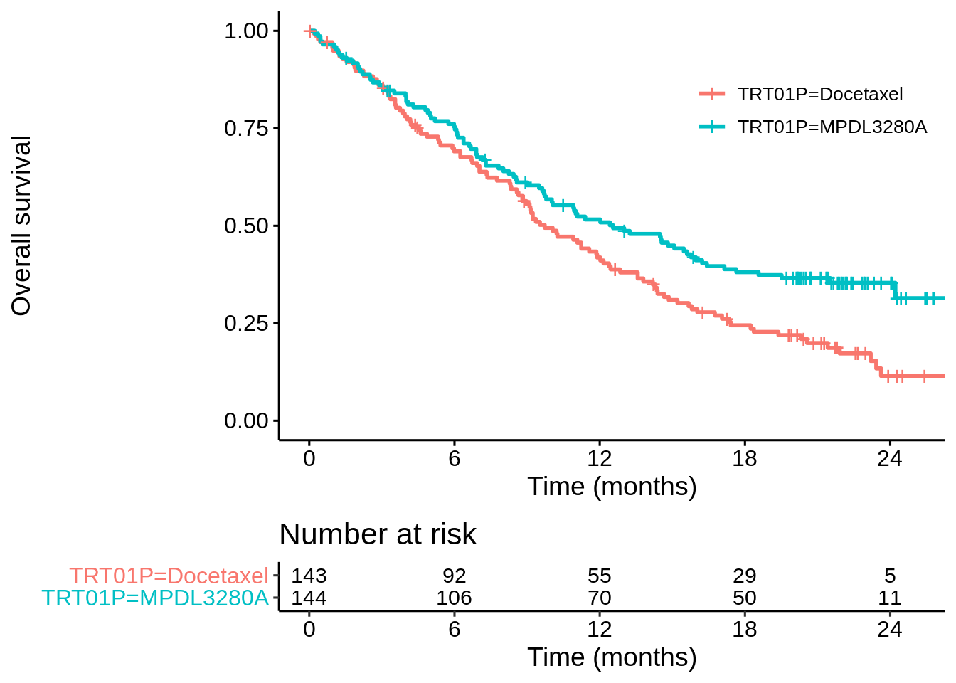
coxph(Surv(OS, OS.EVENT) ~ TRT01P, data = dat_poplar)## Call:
## coxph(formula = Surv(OS, OS.EVENT) ~ TRT01P, data = dat_poplar)
##
## coef exp(coef) se(coef) z p
## TRT01PMPDL3280A -0.3928 0.6752 0.1426 -2.754 0.00589
##
## Likelihood ratio test=7.64 on 1 df, p=0.005724
## n= 287, number of events= 200coxph(Surv(OS, OS.EVENT) ~ TRT01P + ECOGGR, data = dat_poplar)## Call:
## coxph(formula = Surv(OS, OS.EVENT) ~ TRT01P + ECOGGR, data = dat_poplar)
##
## coef exp(coef) se(coef) z p
## TRT01PMPDL3280A -0.3770 0.6859 0.1426 -2.644 0.00819
## ECOGGR 0.4501 1.5684 0.1587 2.836 0.00457
##
## Likelihood ratio test=16.18 on 2 df, p=0.000306
## n= 287, number of events= 200In this case the z-value from the unadjusted Cox model is -2.75, whereas adjusting for ECOGGR it’s -2.644. Let’s look at the un-stratified and stratified modestly-weighted logrank tests (\(t^* = 12\))…
## unstratified
swlrt::wlrt(df = dat_poplar,
            trt_colname = "TRT01P",
            time_colname = "OS",
            event_colname = "OS.EVENT",
            wlr = "mw",
            t_star = 12)
## u v_u z o_minus_e_trt
## 1 -36.83455 134.8164 -3.172372 MPDL3280A## stratified
swlrt::swlrt(df = dat_poplar,
trt_colname = "TRT01P",
time_colname = "OS",
event_colname = "OS.EVENT",
strat_colname = "ECOGGR",
wlr = "mw",
t_star = 12)## $by_strata
## u v_u z o_minus_e_trt
## ECOGGR0 -12.98698 27.30791 -2.485215 MPDL3280A
## ECOGGR1 -20.73634 114.79982 -1.935359 MPDL3280A
##
## $z
## [1] -2.828926Same pattern here, but with lower z-values, as you’d expect given the delayed effect.
Why the different behaviour: OAK vs POPLAR?
This is partly explained from looking at the KM curves by ECOG grade in the two studies. In OAK there is a very big difference in surival (ECOG 1 vs ECOG 0) with the median more-or-less doubling…
km_oak_ecog <- survfit(Surv(OS, OS.EVENT) ~ ECOGGR,
                       data = dat_oak)

survminer::ggsurvplot(km_oak_ecog,
                      data = dat_oak,
                      risk.table = TRUE,
                      break.x.by = 6,
                      legend.title = "",
                      xlab = "Time (months)",
                      ylab = "Overall survival",
                      risk.table.fontsize = 4,
                      legend = c(0.8,0.8))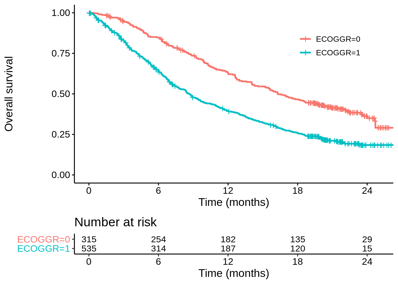
…whereas for POPLAR there is still a clear difference but median only increased by about 33%…
km_poplar_ecog <- survfit(Surv(OS, OS.EVENT) ~ ECOGGR,
                          data = dat_poplar)


survminer::ggsurvplot(km_poplar_ecog,
                      data = dat_poplar,
                      risk.table = TRUE,
                      break.x.by = 6,
                      legend.title = "",
                      xlab = "Time (months)",
                      ylab = "Overall survival",
                      risk.table.fontsize = 4,
                      legend = c(0.8,0.8))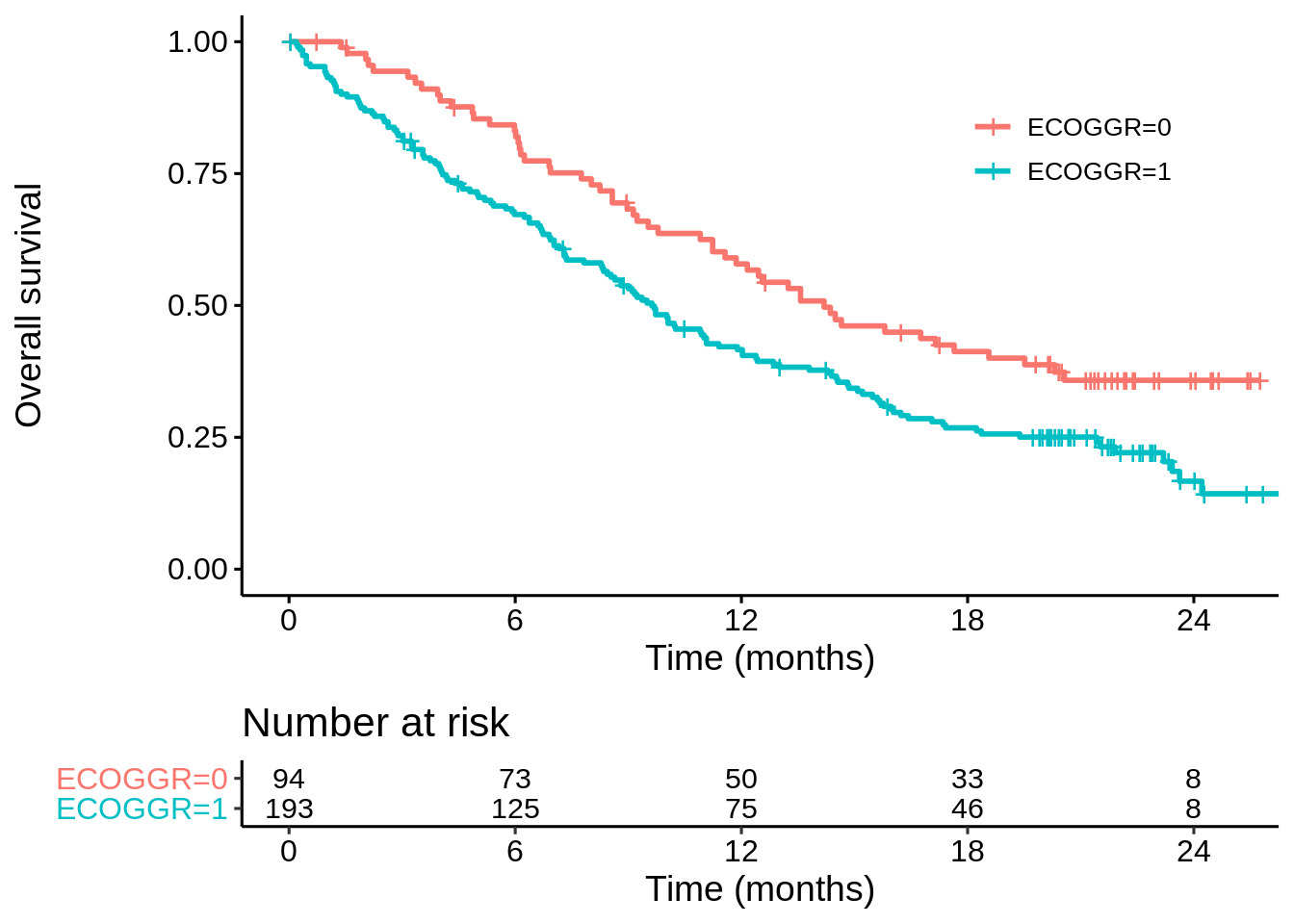
Conclusions
This is just a couple of quick examples, but I think it’s safe to say that if you believe you have a strong prognostic covariate and a delayed treatment effect, then a stratified modestly-weighted logrank test is likely to be a good option in terms of type 1 error and power.
A lot of work has been done on covariate adjustment. Clearly, it’s a complex discussion but I think the consensus is that you are likely to gain more than you lose. A few references I’ve found useful:
https://www.sciencedirect.com/science/article/pii/S0197245697001475
https://www.sciencedirect.com/science/article/pii/S1047279705003248
https://trialsjournal.biomedcentral.com/articles/10.1186/1745-6215-15-139
https://onlinelibrary.wiley.com/doi/full/10.1002/sim.5713
The stratified weighted log-rank test has its limits. It can’t handle continuous covariates, and it’s going to break down when the number of strata becomes too large.
Dominic Magirr
Medical Statistician
Interested in the design, analysis and interpretation of clinical trials.