Landmark/Milestone analysis under a Royston-Parmar flexible parametric survival model using the R package flexsurv
The aim of this post is to demonstrate a landmark/milestone analysis of RCT time-to-event data with a Royston-Parmar flexible parametric survival model. The original reference is:
Royston P, Parmar M (2002). “Flexible Parametric Proportional-Hazards and Proportional-Odds Models for Censored Survival Data, with Application to Prognostic Modelling and Estimation of Treatment Effects.” Statistics in Medicine, 21(1), 2175–2197. doi:10.1002/ sim.1203
This model has been expertly coded and documented by Chris Jackson in the R package flexsurv (https://www.jstatsoft.org/article/view/v070i08). In this post I’ll be making a big meal out of the same material in an effort to increase my own understanding.
I need a dataset, so I’ll re-use one from a previous blogpost – this is publically available data from the OAK RCT comparing a checkpoint inhibitor (MPDL3280A) versus chemotherapy (Docetaxel).
library(survival)
library(dplyr)
library(flexsurv)
dat_oak <- readxl::read_excel("41591_2018_134_MOESM3_ESM.xlsx",
                              sheet = 3) %>%
  select(PtID, ECOGGR, OS, OS.CNSR, TRT01P) %>%
  mutate(OS.EVENT = -1 * (OS.CNSR - 1))

head(dat_oak)
## # A tibble: 6 x 6
## PtID ECOGGR OS OS.CNSR TRT01P OS.EVENT
## <dbl> <dbl> <dbl> <dbl> <chr> <dbl>
## 1 318 1 5.19 0 Docetaxel 1
## 2 1088 0 4.83 0 Docetaxel 1
## 3 345 1 1.94 0 Docetaxel 1
## 4 588 0 24.6 1 Docetaxel 0
## 5 306 1 5.98 0 MPDL3280A 1
## 6 718 1 19.2 1 Docetaxel 0ECOG grade is a prognostic covariate. Initially I’m going to ignore this covariate, but I’ll come back to it later in the post.
I’ll start by plotting the survival curves using the survminer package (https://cran.r-project.org/web/packages/survminer/index.html)…
km_oak <- survfit(Surv(OS, OS.EVENT) ~ TRT01P,
                  data = dat_oak)


survminer::ggsurvplot(km_oak,
                      data = dat_oak,
                      risk.table = TRUE,
                      break.x.by = 6,
                      legend.title = "",
                      xlab = "Time (months)",
                      ylab = "Overall survival",
                      risk.table.fontsize = 4,
                      legend = c(0.8,0.8))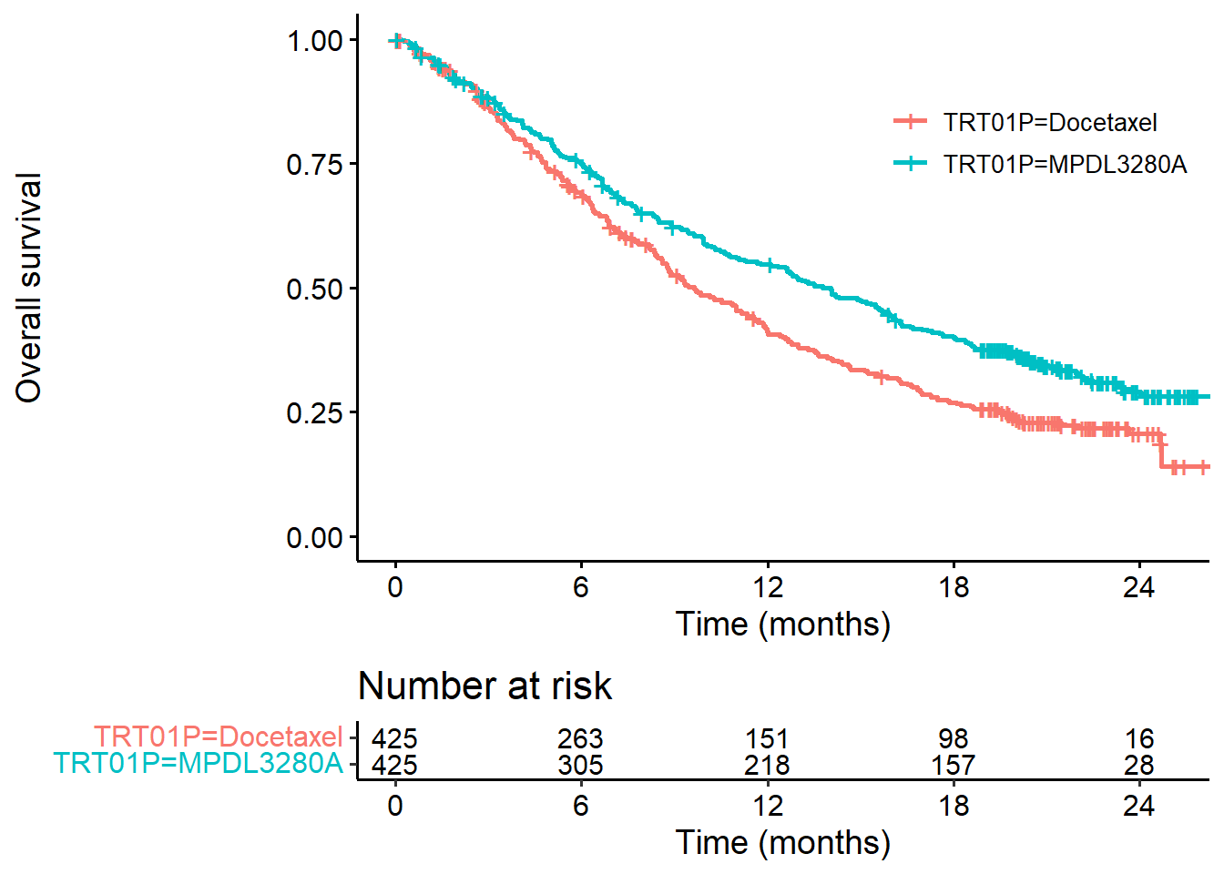
In another previous post I discussed using flexsurv::flexsurvreg to fit a Weibull model. In brief, we can describe this model as two parallel straight lines on the log cumumlative hazard scale (versus log time).
Here, I’ll fit a Weibull model to the OAK data and plot the log cumulative hazard versus log time, on top of the non-parametric equivalent. Note that I’m creating functions here because I’ll want to make this graph repeatedly as we add flexibility to the model.
###########################
### Non-parametric analysis
###########################

# Vector of time in months (for plotting):
t_seq <- seq(1, 24, length.out = 100)
# Extract km estimates
km_sum <- summary(km_oak, times = t_seq, extend = TRUE)

# Function to plot km estimates (log-cumhaz scale)
plot_non_param <- function(){

  plot(log(t_seq), log(km_sum$cumhaz[1:100]), type = "l",
       xlab = "log(time)", ylab = "log cumulative hazard")
  points(log(t_seq), log(km_sum$cumhaz[101:200]), type = "l", col = 2)
  legend("bottomright", c("Docetaxel", "MPDL3280A"),
         lty = c(1,1), col = 1:2)

}

#########################
### Weibull regression
#########################
fit_weibull <- flexsurvreg(Surv(OS, OS.EVENT) ~ TRT01P,
                           data = dat_oak,
                           dist = "weibull")


#Function to add parametric estimate of log-cumulative hazard
#to the KM-based plot
add_model_estimate <- function(fit){

  ### Add Docetaxel estimate
  summary(fit,
          newdata = data.frame(TRT01P = "Docetaxel"),
          t = t_seq, type = "cumhaz")[[1]][,"est"] %>%
    log() %>%
    points(x = log(t_seq), type = "l", lty = 2)

  ### Add MPDL3280A estimate
  summary(fit,
          newdata = data.frame(TRT01P = "MPDL3280A"),
          t = t_seq, type = "cumhaz")[[1]][,"est"] %>%
    log() %>%
    points(x = log(t_seq), type = "l", lty = 2, col = 2)
}


# plot Weibull regression on top of KM estimates
plot_non_param()
add_model_estimate(fit_weibull)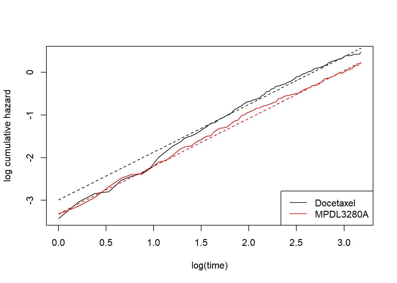
We can see this is not a good fit at early timepoints. Parallel lines on this scale is the same as saying the hazards are proportional, which is clearly not the case. We therefore need to relax the proportional hazards assumption. One option is to maintain the log-cumulative-hazard-versus-log-time perspective, also maintain straight lines on this scale, but give each treatment its own slope. In other words, this is a Weibull model but with a different shape parameter per treatment. One way I could achieve this is to split the data set and fit two separate models. I won’t do this though. Instead I’ll use the flexsurv::flexsurvspline function.
First I’m just going do it. Later I’ll explain the model and syntax.
# spline model with 0 internal knots and where each treatment has its
# own intercept (gamma0) and its own slope (gamma1)
fit_spline_0_1 <- flexsurvspline(Surv(OS, OS.EVENT) ~ TRT01P + gamma1(TRT01P),
                                 data = dat_oak,
                                 k = 0,
                                 scale = "hazard")

plot_non_param()
add_model_estimate(fit_spline_0_1)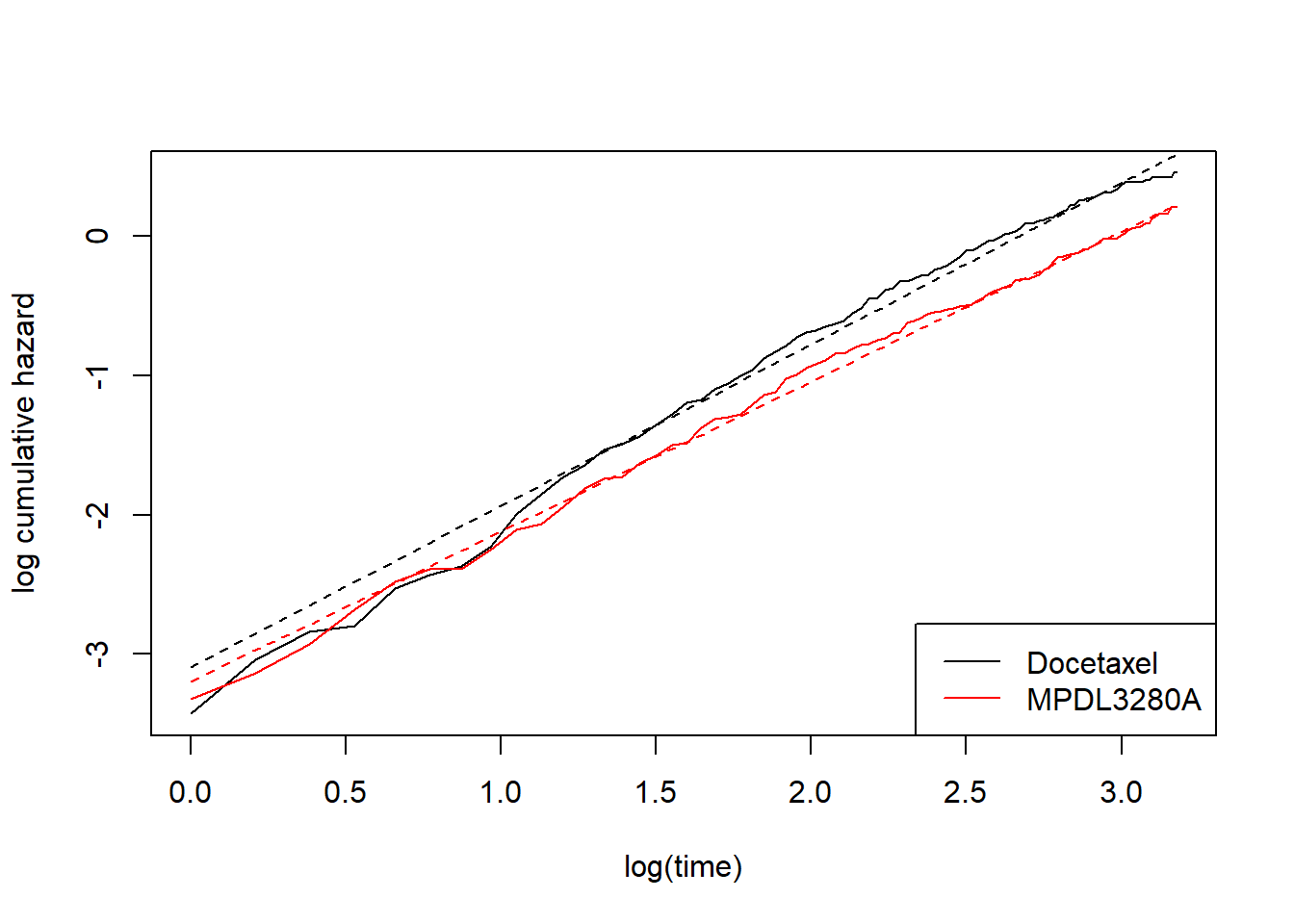
This perhaps looks a bit better, but still not great. At this point we might be tempted to introduce more complex splines. That is, we move away from modelling the log-cumulative hazard versus log time as straight lines. In my previous post I talked about this, but still in the context of a proportional hazards model. That is, allowing curved lines, but proportional. For completeness, this went something like this:
# spline model with 1 internal knot and where each treatment has its
# own intercept (gamma0), but common slope (gamma1) and common gamma2 -- I'll explain later.
fit_spline_1_0 <- flexsurvspline(Surv(OS, OS.EVENT) ~ TRT01P,
                                 data = dat_oak,
                                 k = 1,
                                 scale = "hazard")

plot_non_param()
add_model_estimate(fit_spline_1_0)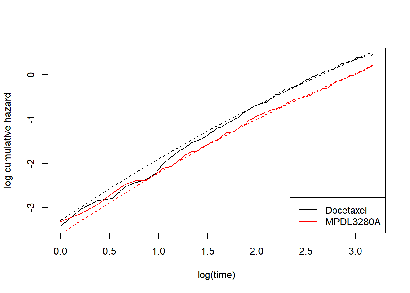
As mentioned, this doesn’t capture the non-proportional hazards. We need something a bit more flexible…
# spline model with 1 internal knot and where each treatment has its
# own intercept (gamma0), its own slope (gamma1), but common gamma2 -- I'll explain later.
fit_spline_1_1 <- flexsurvspline(Surv(OS, OS.EVENT) ~ TRT01P + gamma1(TRT01P),
                               data = dat_oak,
                               k = 1,
                               scale = "hazard")

plot_non_param()
add_model_estimate(fit_spline_1_1)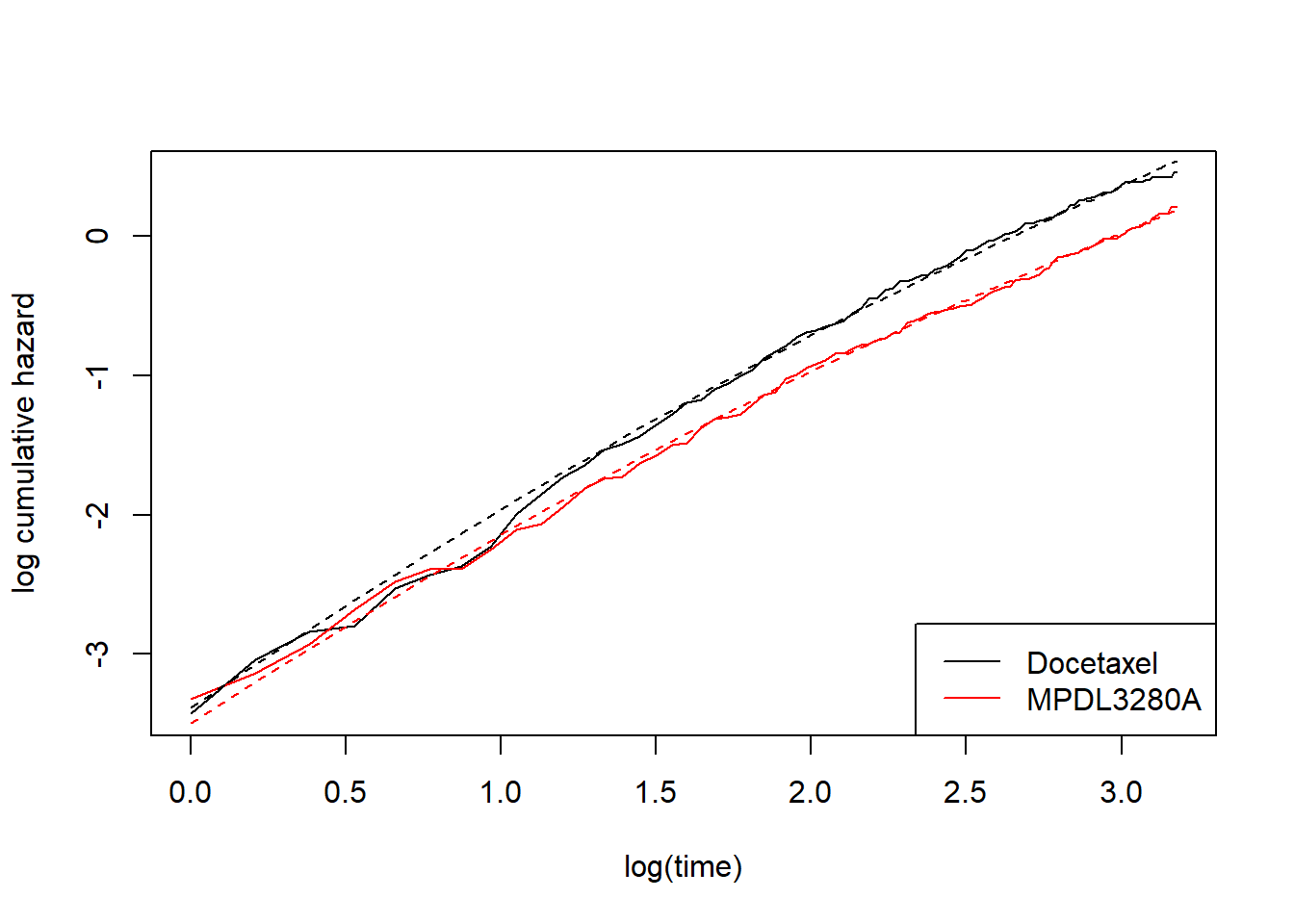
This is starting to look better. Now to expain a bit more what’s going on. Let’s look at the maximum likelihood estimates from the last model:
fit_spline_1_1$res## est L95% U95% se
## gamma0 -3.12264755 -3.44183503 -2.80346006 0.16285375
## gamma1 1.73312765 1.33785579 2.12839950 0.20167302
## gamma2 0.03389207 0.01200609 0.05577806 0.01116653
## TRT01PMPDL3280A -0.10551890 -0.56579074 0.35475295 0.23483689
## gamma1(TRT01PMPDL3280A) -0.07747115 -0.23538127 0.08043896 0.08056787The corresponding model is
\[\log H(t;~Docetaxel) = \gamma_0 + \gamma_1 \times \log(t) + \gamma_2 \times f(\log(t))\] and
\[\log H(t;~MPDL3280A) = \gamma_0 + \text{`TRT01PMPDL3280A`} + \gamma_1 \times \log(t) + \text{`gamma1(TRT01PMPDL3280A)`} \times \log(t) + \gamma_2 \times f(\log(t))\].
Now the question is: what is \(f(\log(t))\)?
The best way to answer that is probably to plot it, together with the other two basis functions (constant and linear) in this model:
my_basis <- flexsurv:::basis(knots = fit_spline_1_1$knots, log(1:24))
my_gamma <- fit_spline_1_1$res[c("gamma0", "gamma1", "gamma2"), "est"]

plot(log(1:24),colSums(t(my_basis) * c(0,0,1)) / -50,
     main = "Basis funs (re-scaled to fit on same plot)",
     xlab = "log(time)",
     ylab = "Arbitrary scale",
     type = "l", ylim = c(-0.5, 1.5))
points(log(1:24),colSums(t(my_basis) * c(0,1,0)) / 3, type = "l", col = 2)
points(log(1:24),colSums(t(my_basis) * c(1,0,0)) , type = "l", col = 3)

legend("bottomright", c("const", "log(t)", "f(log(t))"),
       lty = c(1,1,1),
       col = 3:1)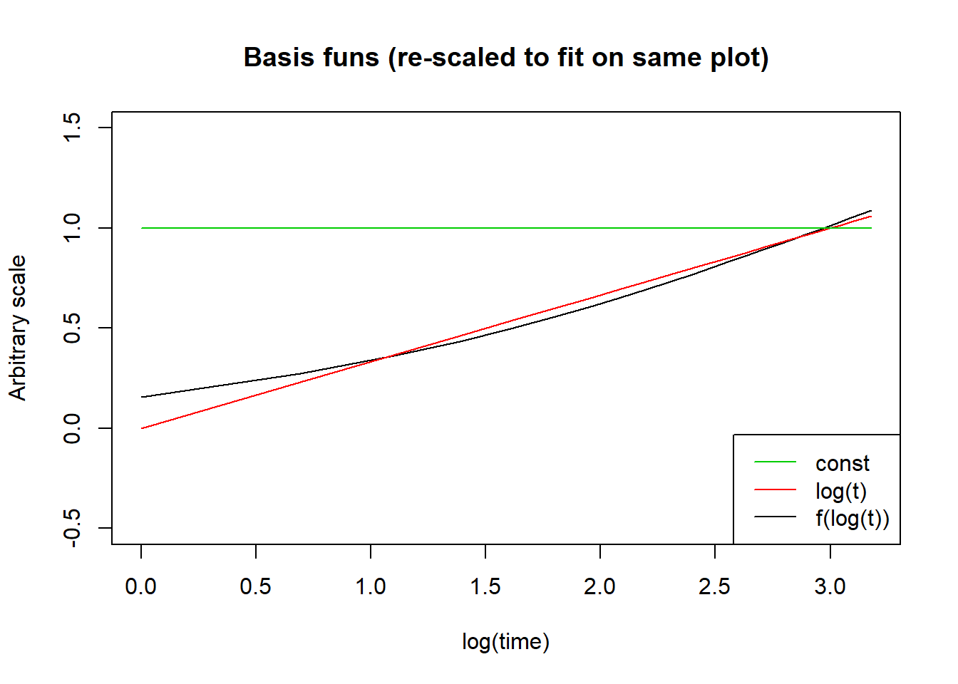
The formulas are given in the flexsurv documentation but I won’t repeat it here because I don’t really care. The important thing is that I’m allowing the log-cumulative hazard function to be a linear combination of more complex basis functions in \(log(t)\).
Hopefully I’ve done enough examples that you can see what the syntax is doing. Basically, by specifying \(k\) internal knots, the baseline log-cumulative hazard is a linear combination of \(k+2\) basis functions, including a constant function, a linear function, and \(k\) more complex things. By default, if you just write something like formula = Surv(OS, OS.EVENT) ~ TRT01P then this will give you a separate constant (gamma0) for each treatment. For the other basis functions, if you want each treatment to have its own version then you must explicitly specify this by adding e.g. gamma1(TRT01P) into the formula. In principle, I don’t see any reason why you couldn’t fit the following model with a common slope (gamma1) but separate gamma2, to give an alternative to fit_spline_1_1 but with the same number of parameters:
# spline model with 1 internal knot and where each treatment has its
# own intercept (gamma0), its own gamma2, but common slope (gamma1).
fit_spline_1_2 <- flexsurvspline(Surv(OS, OS.EVENT) ~ TRT01P + gamma2(TRT01P),
                               data = dat_oak,
                               k = 1,
                               scale = "hazard")

plot_non_param()
add_model_estimate(fit_spline_1_2)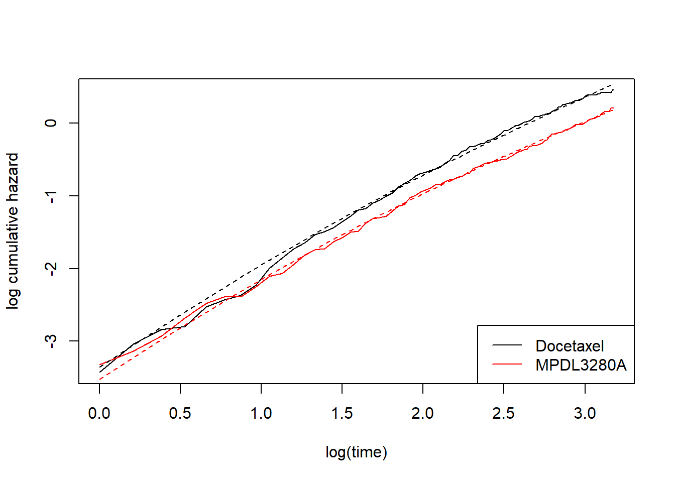
As a final flourish for this post, I’ll do the landmark/milestone analysis based on the model fit_spline_1_1. Let’s pick 18 months as the landmark time. I’ll take the same approach as the flexsurv package. This simulates from the multivariate normal distribution with mean equal to the maximum likelihood estimates and variance equal to the variance of the maximum likelihood estimates. These random draws are then put through a function outputting the quantity of interest (in our case the difference in survival probabilities at 18 months) and we can then take quantiles to give us an estimate and confidence interval.
## simulate from MVN distribution
sims <- normboot.flexsurvreg(fit_spline_1_1,
                             B = 1e5,
                             raw = TRUE)

## give S(18) on docetaxel for each draw
s_18_docetaxel <-  1 - psurvspline(18,
                                   gamma = sims[,c("gamma0", "gamma1", "gamma2")],
                                   knots = fit_spline_1_1$knots)

## give S(18) on MPDL3280A for each draw
s_18_MPDL3280A <-  1 - psurvspline(18,
                                   gamma = cbind(sims[,"gamma0"],
                                                 sims[,"gamma1"]+sims[,"gamma1(TRT01PMPDL3280A)"],
                                                 sims[,"gamma2"]),
                                   offset = sims[,"TRT01PMPDL3280A"],
                                   knots = fit_spline_1_1$knots)

## 95% CI and estimate for diff in survival
## at 18 months (MPDL3280A - docetaxel)
quantile(s_18_MPDL3280A - s_18_docetaxel,
         probs = c(0.025, 0.5, 0.975))
## 2.5% 50% 97.5%
## 0.05959083 0.12016872 0.17982301p.s. prognostic covariate
I promised at one point to discuss the prognostic covariate ECOG status which was available in the data set (in this particular data set it takes values 0 and 1). This post is already longer than I expected, so I won’t dwell on this, but as explained in the flexsurv tutorial it’s possible to do a parametric equivalent of a stratified Cox model by using a spline and allowing each ECOG status to have its own gamma0, gamma1,…,gamma[k+1].
# Make sure ECOGGR is a factor
dat_oak$ECOGGR <- factor(dat_oak$ECOGGR)

# spline model with 2 internal knots and where each ECOG grade has its own
# complex spline, but where treatment effect within strata is a constant shift
fit_spline_ecog_0 <- flexsurvspline(Surv(OS, OS.EVENT) ~ TRT01P +
                                      ECOGGR + gamma1(ECOGGR) + gamma2(ECOGGR) + gamma3(ECOGGR),
                               data = dat_oak,
                               k = 2,
                               scale = "hazard")

fit_spline_ecog_0$res
## est L95% U95% se
## gamma0 -4.39991075 -5.1904477 -3.6093738 0.40334259
## gamma1 2.28385223 0.3406304 4.2270740 0.99145792
## gamma2 -0.02574156 -0.3626805 0.3111974 0.17191077
## gamma3 0.11146845 -0.3340140 0.5569509 0.22729116
## TRT01PMPDL3280A -0.33780623 -0.5033559 -0.1722565 0.08446569
## ECOGGR1 1.63784166 0.7727434 2.5029399 0.44138477
## gamma1(ECOGGR1) -0.85035950 -2.8680837 1.1673647 1.02947003
## gamma2(ECOGGR1) -0.03861271 -0.4030762 0.3258508 0.18595417
## gamma3(ECOGGR1) 0.02669129 -0.4635331 0.5169156 0.25011906This is back to being a proportional hazards model which may not be appropriate. We could then make the treatment effect more flexible, e.g.,
# Make sure ECOGGR is a factor
dat_oak$ECOGGR <- factor(dat_oak$ECOGGR)

# spline model with 2 internal knots and where each ECOG grade has its own
# complex spline, but where treatment effect within strata is handled using a
# constant and linear term only.
fit_spline_ecog_1 <- flexsurvspline(Surv(OS, OS.EVENT) ~ TRT01P + gamma1(TRT01P) +
                                      ECOGGR + gamma1(ECOGGR) + gamma2(ECOGGR) + gamma3(ECOGGR),
                               data = dat_oak,
                               k = 2,
                               scale = "hazard")

fit_spline_ecog_1$res
## est L95% U95% se
## gamma0 -4.524045821 -5.3443397 -3.70375194 0.41852498
## gamma1 2.296987159 0.3559155 4.23805878 0.99036086
## gamma2 -0.030850110 -0.3674476 0.30574735 0.17173655
## gamma3 0.117629309 -0.3273831 0.56264169 0.22705131
## TRT01PMPDL3280A -0.085983706 -0.5482385 0.37627105 0.23584859
## ECOGGR1 1.660089705 0.7948724 2.52530704 0.44144553
## gamma1(TRT01PMPDL3280A) -0.093731710 -0.2545742 0.06711074 0.08206398
## gamma1(ECOGGR1) -0.799217529 -2.8168457 1.21841060 1.02942102
## gamma2(ECOGGR1) -0.024330400 -0.3890199 0.34035906 0.18606947
## gamma3(ECOGGR1) 0.006536356 -0.4839968 0.49706953 0.25027663It then becomes difficult to summarise the treatment effect succinctly. This is an interesting but complicated topic that I won’t discuss now.
Dominic Magirr
Medical Statistician
Interested in the design, analysis and interpretation of clinical trials.