Longitudinal hurdle models

Data

Recently, I have been modelling data that is longitudinal, contains excess zeros, and where the non-zero data is right-skewed and measured on a continuous scale, rather than being count data.

I’ll simulate a semi-realistic example data set from a lognormal hurdle model. The “random effects” for the pr(zero) and non-zero parts of the model are negatively correlated.

set.seed(180)

## 100 patients
id <- 1:100

## 2 timepoints
time <- c("1", "2")

## random effects
u <- rnorm(100, sd = 2)
v <- rnorm(100, mean = -0.95 * u, sd = sqrt((1 - 0.95^2) * 4)) # p(zero) is negatively correlated with Y*

## non-zero data (4 obs per id, at two timepoints)
ystar1 <- exp(rnorm(400, mean = u, sd = 1))
ystar2 <- exp(rnorm(400, mean = -0.5 + u, sd = 1))

## z = 1 if "cross hurdle", i.e. if not zero
z1 <- rbinom(400, size = 1, prob = 1 - plogis(-2 + v)) # p(cross hurdle) = 1 - p(zero)
z2 <- rbinom(400, size = 1, prob = 1 - plogis(-1 + v))

dat <- data.frame(y = c(z1 * ystar1, z2 * ystar2),
                  time = rep(time, each = 400),
                  id = rep(id, 8))

In this data set there are 100 patients and two timepoints. For each patient, at each timepoint, I have simulated 4 independent observations (I’ve only done this to make model convergence a bit easier). The important point is that the data is correlated within patient, and also z (hurdle part) and ystar (non-zero part) are correlated, so that patients who start with a smaller (non-zero) y at the first timepoint are more likely to have y = 0 at the second timepoint. This can be clearly seen in the plot below.

library(tidyverse)
ggplot(data = dat,
                mapping = aes(x = time, y = y, group = id)) +
  geom_point() +
  geom_line() +
  scale_y_log10()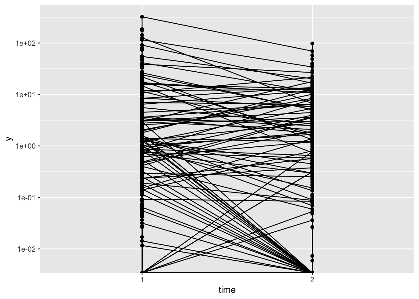

Fit the model

To fit the model I’m using the excellent brms package (https://github.com/paul-buerkner/brms)

Bürkner P. C. (2018). Advanced Bayesian Multilevel Modeling with the R Package brms. The R Journal. 10(1), 395-411. doi.org/10.32614/RJ-2018-017

library(brms)

fit_hurdle <- brm(bf(y ~  time + (1 | q | id),
                     hu ~ time + (1 | q | id)),
                  data = dat,
                  iter = 4000,
                  family = hurdle_lognormal(),
                  refresh = 0)

summary(fit_hurdle)

##  Family: hurdle_lognormal 
##   Links: mu = identity; sigma = identity; hu = logit 
## Formula: y ~ time + (1 | q | id) 
##          hu ~ time + (1 | q | id)
##    Data: dat (Number of observations: 800) 
## Samples: 4 chains, each with iter = 4000; warmup = 2000; thin = 1;
##          total post-warmup samples = 8000
## 
## Group-Level Effects: 
## ~id (Number of levels: 100) 
##                             Estimate Est.Error l-95% CI u-95% CI Rhat
## sd(Intercept)                   1.96      0.16     1.69     2.29 1.00
## sd(hu_Intercept)                2.47      0.30     1.93     3.11 1.00
## cor(Intercept,hu_Intercept)    -0.90      0.04    -0.97    -0.81 1.00
##                             Bulk_ESS Tail_ESS
## sd(Intercept)                   1452     2688
## sd(hu_Intercept)                2979     5484
## cor(Intercept,hu_Intercept)     2539     4394
## 
## Population-Level Effects: 
##              Estimate Est.Error l-95% CI u-95% CI Rhat Bulk_ESS Tail_ESS
## Intercept        0.07      0.20    -0.34     0.45 1.00      885     1970
## hu_Intercept    -2.72      0.34    -3.43    -2.07 1.00     1662     3089
## time2           -0.33      0.08    -0.49    -0.18 1.00    14798     5985
## hu_time2         1.26      0.24     0.80     1.73 1.00    12452     5627
## 
## Family Specific Parameters: 
##       Estimate Est.Error l-95% CI u-95% CI Rhat Bulk_ESS Tail_ESS
## sigma     0.94      0.03     0.88     1.00 1.00    11293     6175
## 
## Samples were drawn using sampling(NUTS). For each parameter, Eff.Sample 
## is a crude measure of effective sample size, and Rhat is the potential 
## scale reduction factor on split chains (at convergence, Rhat = 1).

Inference

From the output I can see that I have more-or-less recovered the parameters from my model. In practice, I could use this to make inference on the two parts of the model separately. In future posts I’ll discuss how to make inference/predictions when combining the two parts of the model.