That'll do: simulated annealing instead of maths
This is a post for future me. Given my steadily declining maths skills, I can see myself needing to use the generalized simulated annealing function GenSA::GenSA a lot more.
For example, suppose I’m helping to design a clinical trial and I want to simulate some data from a Gompertz distribution. I know that the Gompertz distribution allows a rapidly decreasing hazard function (that’s why I want to use it), but I’m not familiar with the details, and don’t have the time/motivation right now to do any maths. I want the survival probability at 1 month to be about 80%, at 3 months to be about 75%, and at 12 months to be about 65%. What are the corresponding parameters of the Gompertz distribution?
From looking at the help pages ?flexsurv::pgompertz, i see that the Gompertz has a shape parameter a and a rate parameter b. I write a quick function to calculate the distance between a Gompertz(a,b) distribution and my desired milestone probabilities:
gomp_close <- function(a_b,
                       t_1, ## timepoint 1
                       t_2, ## timepoint 1
                       t_3, ## timepoint 2
                       p_1, ## p(event by t_1)
                       p_2,
                       p_3){

  a <- a_b[1]
  b <- a_b[2]

  distance_1 <- flexsurv::pgompertz(t_1, a, b) - p_1
  distance_2 <- flexsurv::pgompertz(t_2, a, b) - p_2
  distance_3 <- flexsurv::pgompertz(t_3, a, b) - p_3

  distance_1 ^ 2 + distance_2 ^ 2 + distance_3 ^ 2

}
and then I let the simulated annealing function find a close enough solution:
result <- GenSA::GenSA(par = c(1, 1), # initial values
                       fn = gomp_close,
                       lower = c(-100, 0), # parameter b is positive, so lower lim 0
                       upper = c(100, 100),
                       t_1 = 1,
                       t_2 = 3,
                       t_3 = 12,
                       p_1 = 0.2,
                       p_2 = 0.25,
                       p_3 = 0.35)

result$par
## [1] -0.6307335 0.2536741Just check this looks ok:
x <- seq(0, 24, length.out = 100)
s <- flexsurv::pgompertz(x,
                         shape = result$par[1],
                         rate = result$par[2],
                         lower.tail = FALSE)

plot(x, s, type = "l", ylim = c(0,1))
points(c(1, 3, 12), c(0.8, 0.75, 0.65))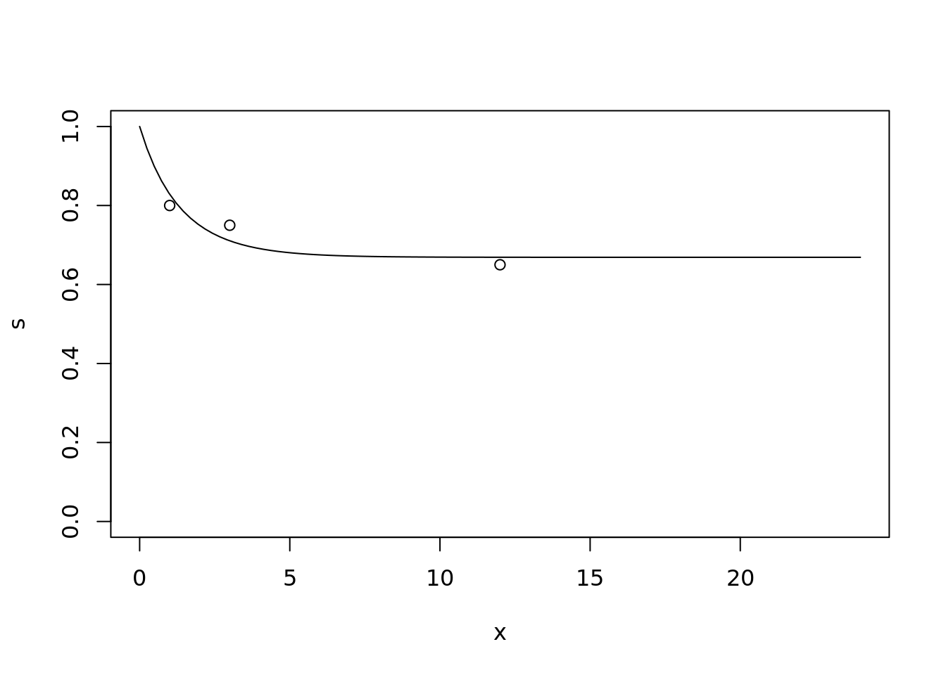
Dominic Magirr
Medical Statistician
Interested in the design, analysis and interpretation of clinical trials.