The MaxCombo Test severely inflates the type 1 error rate
“The MaxCombo Test severely inflates the type 1 error rate”, by Carl-Fredrik Burman and myself has just been published in JAMA Oncology.
It’s our reaction to
The central idea in Mukhopadhyay et al is that in many immuno-oncology trials, for example when a new immunotherapy is compared with chemotherapy, we see a delayed separation of overall survival curves. Sometimes, the results from a standard Cox model or log-rank test are not significant at an alpha level typically required for confirmatory trials. But we see a clear indication of long-term survival benefit. If we used weighted log-rank tests instead that give more weight to later events, then more of theses cases would be statistically significant. Based on a review of 63 studies, the authors found that the results of the log-rank test and a particular type of weighted log-rank test (the MaxCombo test) were concordant in 90% of cases, but in 10% of cases the MaxCombo test was significant while the log-rank test wasn’t.
Broadly speaking, we agree with this perspective. But the devil is in the detail. The MaxCombo test gives extremely low weights to early events. So much so, in fact, that the test statistic ends up “rewarding” the experimental treatment for causing early harm, and “punishing” the experimental treatment for causing early benefit.
Mukhopadhyay et al make the following statement:
“It is critical that a statistical test control for type I (false-positive) error. Based on a previous review [19] the modified MaxCombo, which has been applied here, will control for type I error even in extreme scenarios [30,31] (eg, the hypothetical scenario in Freidlin and Korn [30] where the HR was 3.53 in the first 6 months and 0.75 beyond 6 months).”
We completely disagree. Hence the title of our letter. In fact, reference [31] is the first paper we wrote to show what can go wrong when the weights in a weighted log-rank test are not carefully chosen. Something we have pointed out repeatedly.
In the past, we have tried to demonstrate the problem with simulation studies. It is easy to find scenarios where survival is worse on the experimental treatment than control, yet there is a substantial probability of the MaxCombo test concluding the opposite. This message has clearly not worked.
So in this letter we try a different approach. We build on the case study in Mukhopadhyay et al. (their Figure 2), where
“there was a modest crossing [of survival curves] during the first 4 months […], there was a clinically meaningful overall treatment benefit with HR of 0.74 (95% CI, 0.54-1.02). However, log-rank test failed to reach nominal significance in this case, while both MaxCombo 2 and MaxCombo 3 did.”
Having (approximately) recovered the data, let’s reproduce the Kaplan-Meier curves:
library(survival)
library(ggplot2)
library(dplyr)
## get data set
dat <- read.csv("https://github.com/dominicmagirr/max_combo_ex/raw/main/moderate_cross.csv")
## plot data
km <- survfit(Surv(time, event) ~ arm, data = dat)
p_dat <- survminer::ggsurvplot(km,
data = dat,
risk.table = TRUE,
break.x.by = 6,
legend.title = "",
xlab = "Time (months)",
ylab = "Overall survival",
risk.table.fontsize = 4,
legend = c(0.8,0.8),
title = "Data Set 1")
p_dat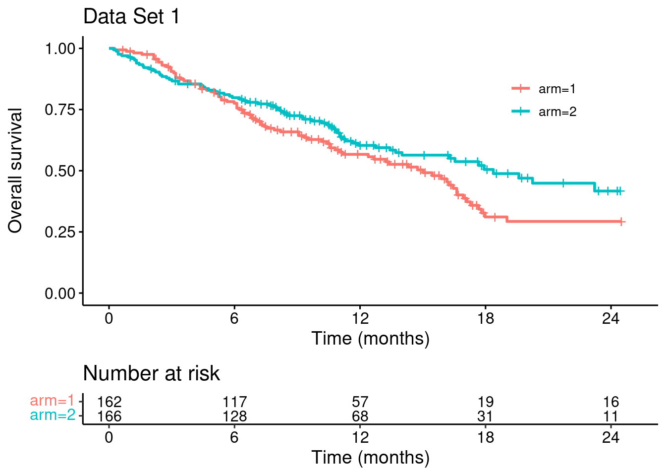
To make the problems with the MaxCombo test explicit, we modify this dataset such that the survival curves match for the first four months (keeping everything else unchanged)…
## modify data set...
dat_1_pre <- dat[dat$time <= 4 & dat$arm == 1,]
dat_2_pre <- dat_1_pre
dat_2_pre$arm = 2
dat_post <- dat[dat$time > 4,]
dat_new <- rbind(dat_1_pre, dat_2_pre, dat_post)

## plot datasets (orginal vs modified)
km_new <- survfit(Surv(time, event) ~ arm, data = dat_new)
p_dat_new <- survminer::ggsurvplot(km_new,
                               data = dat_new,
                               risk.table = TRUE,
                               break.x.by = 6,
                               legend.title = "",
                               xlab = "Time (months)",
                               ylab = "Overall survival",
                               risk.table.fontsize = 4,
                               legend = c(0.8,0.8),
                               title = "Data Set 2")

survminer::arrange_ggsurvplots(list(p_dat, p_dat_new))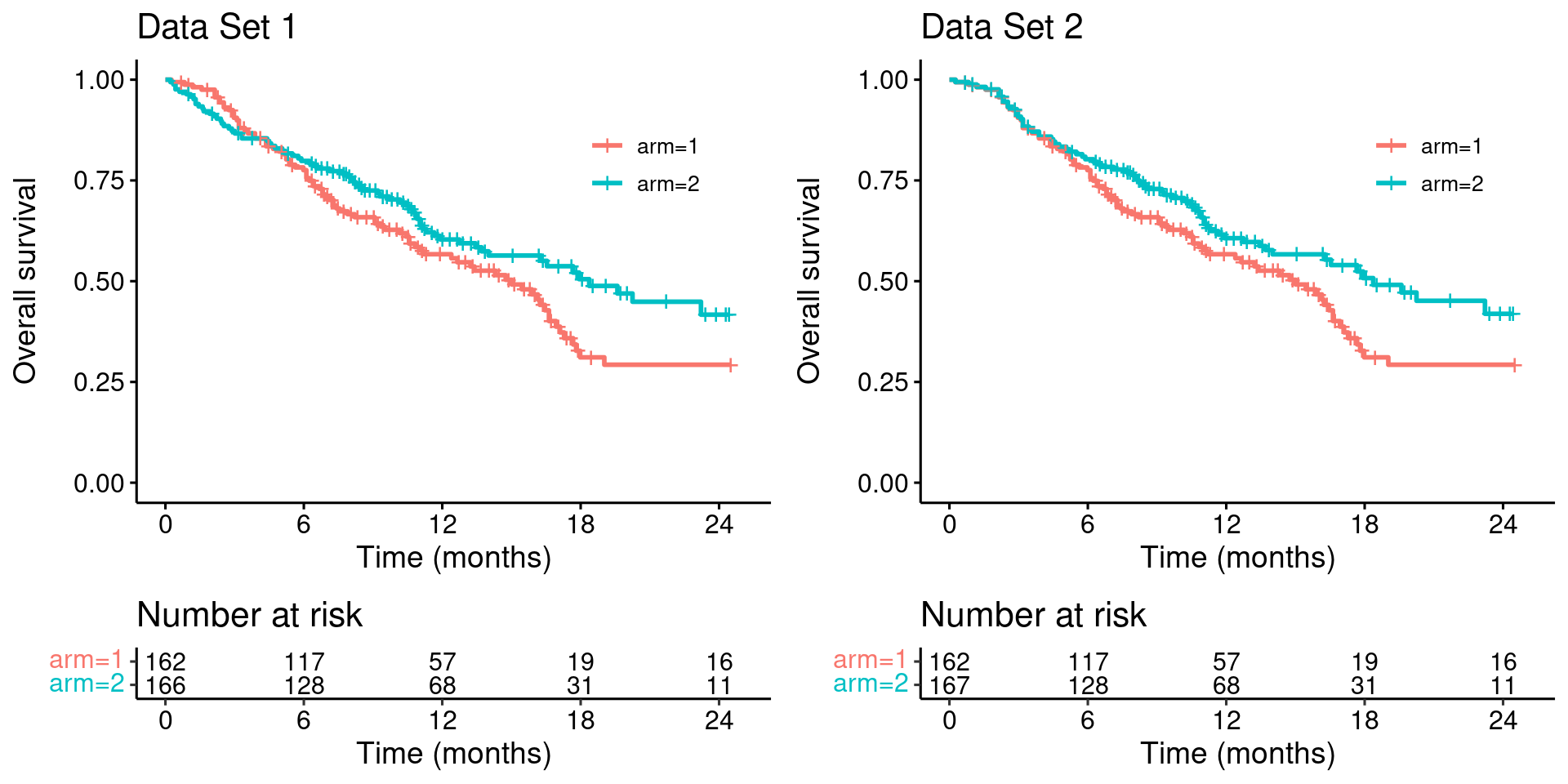
Looking at these two plots side-by-side it is clear that Data Set 1 does not constitute stronger evidence for the benefit of the experimental treatment (arm 2), compared with the Data Set 2.
Let’s now try some hypothesis tests.
Log-rank test
We’ll use the excellent {nph} package by Ristl et al. Firstly, the standard log-rank test
library(nph)# Data set 1
logrank.test(
time = dat$time,
event = dat$event,
group = dat$arm,
rho = c(0),
gamma = c(0)
)## Call:
## logrank.test(time = dat$time, event = dat$event, group = dat$arm,
## rho = c(0), gamma = c(0))
##
## N Observed Expected (O-E)^2/E (O-E)^2/V
## 1 162 84 72.9 1.68 3.19
## 2 166 71 82.1 1.49 3.19
##
## Chisq= 3.2 on 1 degrees of freedom, p= 0.07
## rho = 0 gamma = 0So, for Data Set 1, the observed - expected number of events on arm 1 is 84 - 72.9, with Z-statistic sqrt(3.19)=1.786, one-sided p-value 1 - pnorm(1.786)=0.037, and two-sided p-value 0.07.
Now, for Data Set 2…
# Data set 2
logrank.test(
  time  = dat_new$time,
  event = dat_new$event,
  group = dat_new$arm,
  rho   = c(0),
  gamma = c(0)
)
## Call:
## logrank.test(time = dat_new$time, event = dat_new$event, group = dat_new$arm,
## rho = c(0), gamma = c(0))
##
## N Observed Expected (O-E)^2/E (O-E)^2/V
## 1 162 84 72 2.00 3.78
## 2 167 70 82 1.75 3.78
##
## Chisq= 3.8 on 1 degrees of freedom, p= 0.05
## rho = 0 gamma = 0the observed - expected number of events is 84 - 72, with Z-statistic sqrt(3.78)=1.944, one-sided p-value 1 - pnorm(1.944)=0.026, and two-sided p-value 0.05.
This makes complete sense. The results in Data Set 1 are not better than in Data Set 2.
MaxCombo test
The version of the MaxCombo test recommended by Mukhopadhyay et al is the maximum of the standard log-rank test and the Fleming-Harrington-(0, 0.5) test. Let’s try it out…
# Data set 1
logrank.maxtest(
  time  = dat$time,
  event = dat$event,
  group = dat$arm,
  rho   = c(0, 0),
  gamma = c(0, 0.5)
)
## Call:
## logrank.maxtest(time = dat$time, event = dat$event, group = dat$arm,
## rho = c(0, 0), gamma = c(0, 0.5))
##
## Two sided p-value = 0.0289 (Bonferroni corrected: 0.0418)
##
## Individual weighted log-rank tests:
## Test z p
## 1 1 1.79 0.0741
## 2 2 2.31 0.0209For Data Set 1 the two-sided p-value is 0.0289. This is a multiplicity corrected p-value (since we are taking the maximum of two statistics), but we can see that it is driven by the large z-value z = 2.31 from the second statistic – the Fleming-Harrington-(0,0.5) statistic.
When we try this on Data Set 2…
# Data set 2
logrank.maxtest(
  time  = dat_new$time,
  event = dat_new$event,
  group = dat_new$arm,
  rho   = c(0, 0),
  gamma = c(0, 0.5)
)
## Call:
## logrank.maxtest(time = dat_new$time, event = dat_new$event, group = dat_new$arm,
## rho = c(0, 0), gamma = c(0, 0.5))
##
## Two sided p-value = 0.0457 (Bonferroni corrected: 0.0669)
##
## Individual weighted log-rank tests:
## Test z p
## 1 1 1.94 0.0519
## 2 2 2.13 0.0335… the two-sided p-value is 0.0457 driven by a Fleming-Harrington-(0,0.5) z-value of 2.13.
Hang on a second! We’ve agreed that the results in Data Set 1 are not ‘better’ than the results in Data Set 2. Yet the p-value is lower, 0.03 compared with 0.05.
Remember the context. Mukhopadhyay et al are using this as a case study for when the log-rank statistic is not statistically significant but the MaxCombo test is. However, we now see that this happens (partly) by the test statistic “rewarding” an early detrimental effect on survival.
What’s going on?
The Fleming-Harrington-(0,0.5) test gives extremely low weights to early events.
Remember that the weighted log-rank statistic is
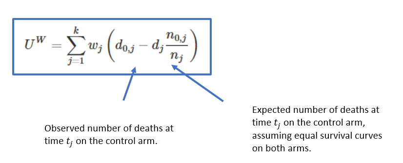
Let’s plot the weights for the original data set, for which I’ll use {nphRCT}
library(nphRCT)## At-risk table
at_risk <- nphRCT::find_at_risk(Surv(time, event) ~ arm,
data = dat,
include_cens = FALSE)
## F-H-(0,0.5) weights
weights_fh <- nphRCT::find_weights(Surv(time, event) ~ arm,
data = dat,
method = "fh",
rho = 0,
gamma = 0.5)
plot(at_risk$t_j, weights_fh, ylim = c(0,1),
xlab = "Event time",
ylab = "Weight",
main = "Fleming-Harrington (0,0.5)")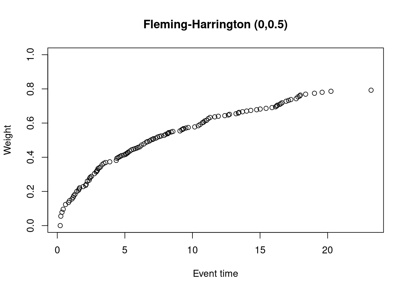
Alternative visualization of a weighted log-rank test
It’s possible to visualize a (weighted) log-rank test as a difference in mean “score” on the two treatment arms, where the scores are a transformation of the 2-dimensional outcomes (time, event status) to the real line. This is explained in more detail here.
We’ll try it now for Data Set 1. In the following plots, each dot corresponds to a patient in the trial. On the x-axis is their time-to-event/censoring, and on the y-axis is their score. For the log-rank test, we see two almost parallel lines, with the top line corresponding to the observed events, and the bottom line corresponding to censored observations. So someone who dies at month 1 gets a score close to 1 (the worst score), and someone who is censored at month 24 gets a score close to -1 (the best score). Note that the scaling is arbitrary. The dashed horizontal lines represent the mean score on the two treatment arms. The difference between these to lines is the log-rank test statistic (a re-scaled version of it).
# Standard log-rank test
nphRCT::find_scores(Surv(time, event) ~ arm,
             data = dat,
             method = "lr") %>%
  plot() +
  ggtitle("Standard log-rank test")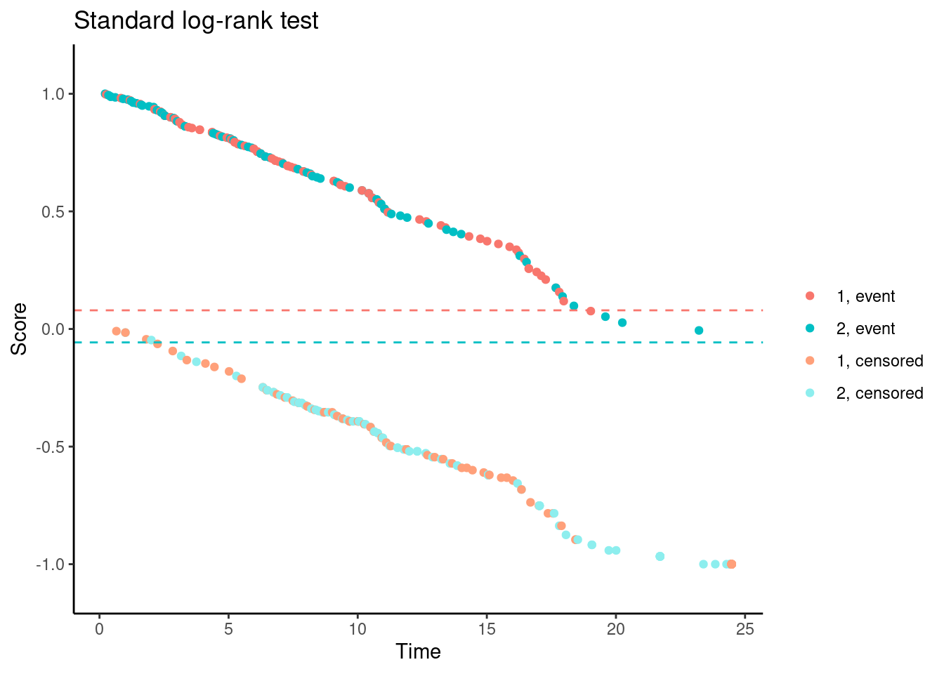
In contrast, for the Fleming-Harrington-(0,0.5) test, the scores (for observed events) are increasing with time for early follow-up times. So someone who dies at month 1 gets a lower (better) score than someone who dies at month 12. Basically, one has downweighted the early events to such an extent that the test actually “rewards” the experimental treatment for causing early harm.
# Fleming-Harrington (0,0.5)
nphRCT::find_scores(Surv(time, event) ~ arm,
             data = dat,
             method = "fh",
             rho = 0,
             gamma = 0.5) %>%
  plot() +
  ggtitle("Fleming-Harrington (0,0.5)")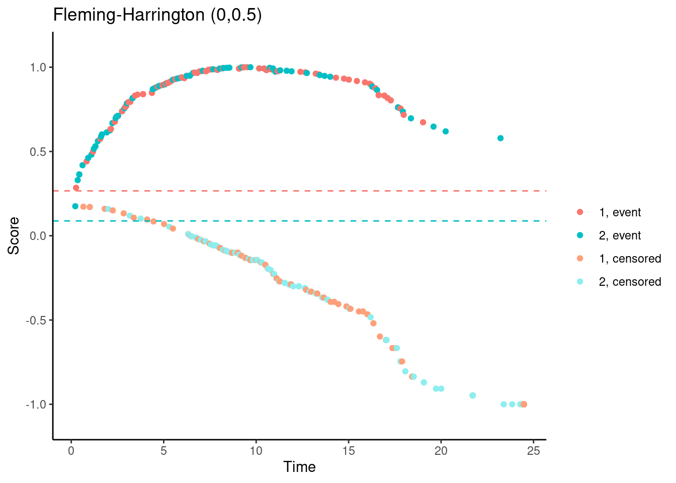
Modestly-weighted tests
One possible approach that we favour is a modestly-weighted test. We won’t go into the full details again here, but essentially we can give later events higher weight than earlier events (notice that the first weight is 1 rather than 0)…
weights_mw_s <- nphRCT::find_weights(Surv(time, event) ~ arm,
                                     data = dat,
                                     method = "mw",
                                     s_star = 0.5)


plot(at_risk$t_j, weights_mw_s, ylim = c(0,2),
     xlab = "Event time",
     ylab = "Weight",
     main = "Modestly weighted, s*=0.5")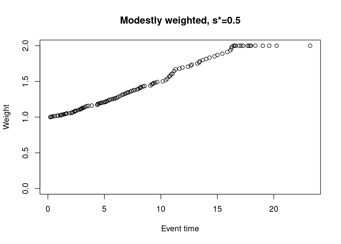
while still ensuring that the scores are not increasing for early follow-up times…
# Modestly-weighted (s*=0.5)
nphRCT::find_scores(Surv(time, event) ~ arm,
             data = dat,
             method = "mw",
             s_star = 0.5) %>%
  plot() +
  ggtitle("Modestly-weighted (s*=0.5)")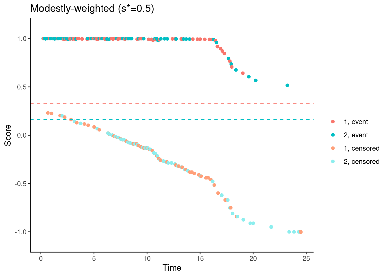
References
Mukhopadhyay, Pralay, Jiabu Ye, Keaven M. Anderson, Satrajit Roychoudhury, Eric H. Rubin, Susan Halabi, and Richard J. Chappell. “Log-Rank Test vs MaxCombo and Difference in Restricted Mean Survival Time Tests for Comparing Survival Under Nonproportional Hazards in Immuno-oncology Trials: A Systematic Review and Meta-analysis.” JAMA oncology (2022).
Magirr, Dominic, and Carl‐Fredrik Burman. “Modestly weighted logrank tests.” Statistics in medicine 38, no. 20 (2019): 3782-3790.
Magirr, Dominic, and Carl-Fredrik Burman. “The Strong Null Hypothesis and the MaxCombo Test: Comment on “Robust Design and Analysis of Clinical Trials with Nonproportional Hazards: A Straw Man Guidance form a Cross-Pharma Working Group.”.” Statistics in Biopharmaceutical Research (2021): 1-2.
Ristl, Robin, Nicolás M. Ballarini, Heiko Götte, Armin Schüler, Martin Posch, and Franz König. “Delayed treatment effects, treatment switching and heterogeneous patient populations: How to design and analyze RCTs in oncology.” Pharmaceutical statistics 20, no. 1 (2021): 129-145.
Dominic Magirr
Medical Statistician
Interested in the design, analysis and interpretation of clinical trials.