flexsurv 2

From Weibull regression to Cox regression.

For a Weibull distribution with shape \(a\), scale \(b\), covariates \(x\), and regression coefficents \(\gamma\), the survival probability is

\[S(t; x) = \exp\left\lbrace - \left( \frac{t}{b \cdot \exp(x^T\gamma)} \right) ^ a\right\rbrace\]

Since survival is related to the log-cumulative hazard via \(S=\exp(-H)\), this means that

\[\log H(t;x) = a\log t - a\log(b) - a x^T\gamma\]

In words, the log-cumulative hazard has a linear relationship with (log-) time, with the intercept depending on the value of \(x\). For a given data set, we can check if this is reasonable by looking at non-paramteric estimates, \(\log \hat{H}(t; x)\).

library(survival)
library(flexsurv)
library(ggplot2)

### Non-parametric analysis
fit_km <- survfit(Surv(futime, death) ~ trt,
                  data = myeloid)
t_seq <- seq(1, 2500, length.out = 1000)
km_sum <- summary(fit_km, times = t_seq, extend = TRUE)

### Weibull regression
fit_weibull <- flexsurvreg(Surv(futime, death) ~ trt, 
                           dist = "weibull", 
                           data = myeloid)

a <- fit_weibull$res["shape", "est"]
b <- fit_weibull$res["scale", "est"]
trtB <- fit_weibull$res["trtB", "est"]


### plot log-cumulative hazard against log-time
df <- data.frame(log_time = log(rep(t_seq, 2)),
                 logcumhaz = log(-log(km_sum$surv)),
                 trt = rep(c("A", "B"), each = 1000),
                 logcumhaz_w = c(a * (log(t_seq) - log(b)),
                                 a * (log(t_seq) - log(b) - trtB)))

ggplot(data = df,
       mapping = aes(x = log_time,
                     y = logcumhaz,
                     colour = trt)) +
  geom_line() +
  geom_line(mapping = aes(x = log_time,
                          y = logcumhaz_w,
                          colour = trt),
            linetype = 2) +
  theme_bw() +
  scale_x_continuous(limits = c(2,8)) +
  scale_y_continuous(limits = c(-6,0))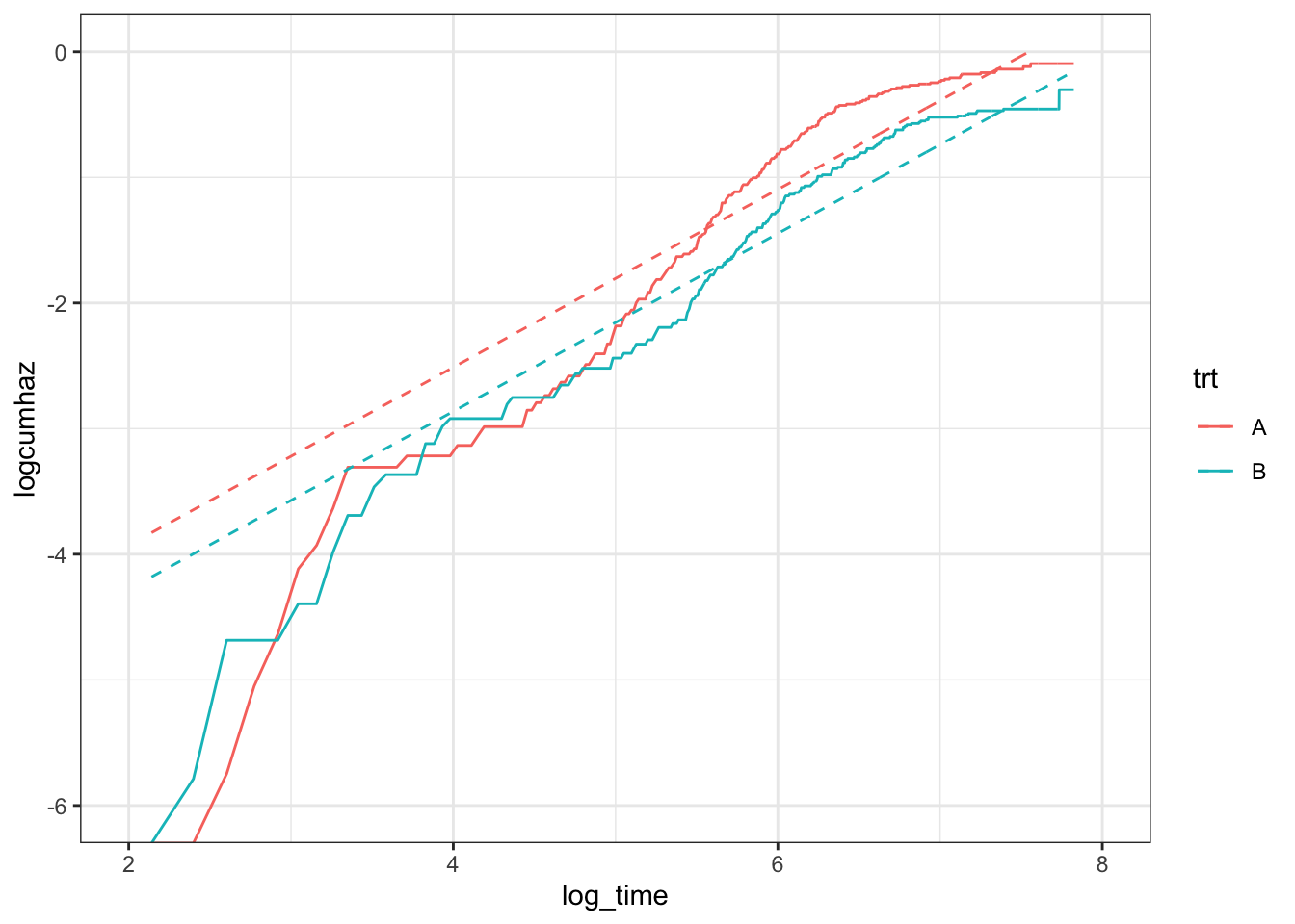

What’s going on here? Well, the first thing to acknowledge is that the hazards only appear to be proportional after about 150 (\(e^5\)) days. I’m not sure I would immediately abandon a proportional-hazards model, though, as most of the events happen when the hazards are proportional (only 10-15% of the events happen before day 150), so the right-hand-side of the plot is far more important. Looking to the right then: the relationship between the log-cumulative hazard and log-time is not really linear. The distance between the two lines is roughly the same for the two models (Weibull and non-parametric), suggesting that the Weibull model does ok at estimating the hazard ratio. However, the lack of linearity will lead to poor estimates for the medians, \(P(S>s^*)\), etc., as can be confirmed by plotting the survival curves:

ggplot(data = df,
       mapping = aes(x = exp(log_time),
                     y = exp(-exp(logcumhaz)),
                     colour = trt)) +
  geom_line() +
  geom_line(mapping = aes(x = exp(log_time),
                          y = exp(-exp(logcumhaz_w)),
                          colour = trt),
            linetype = 2) +
  theme_bw()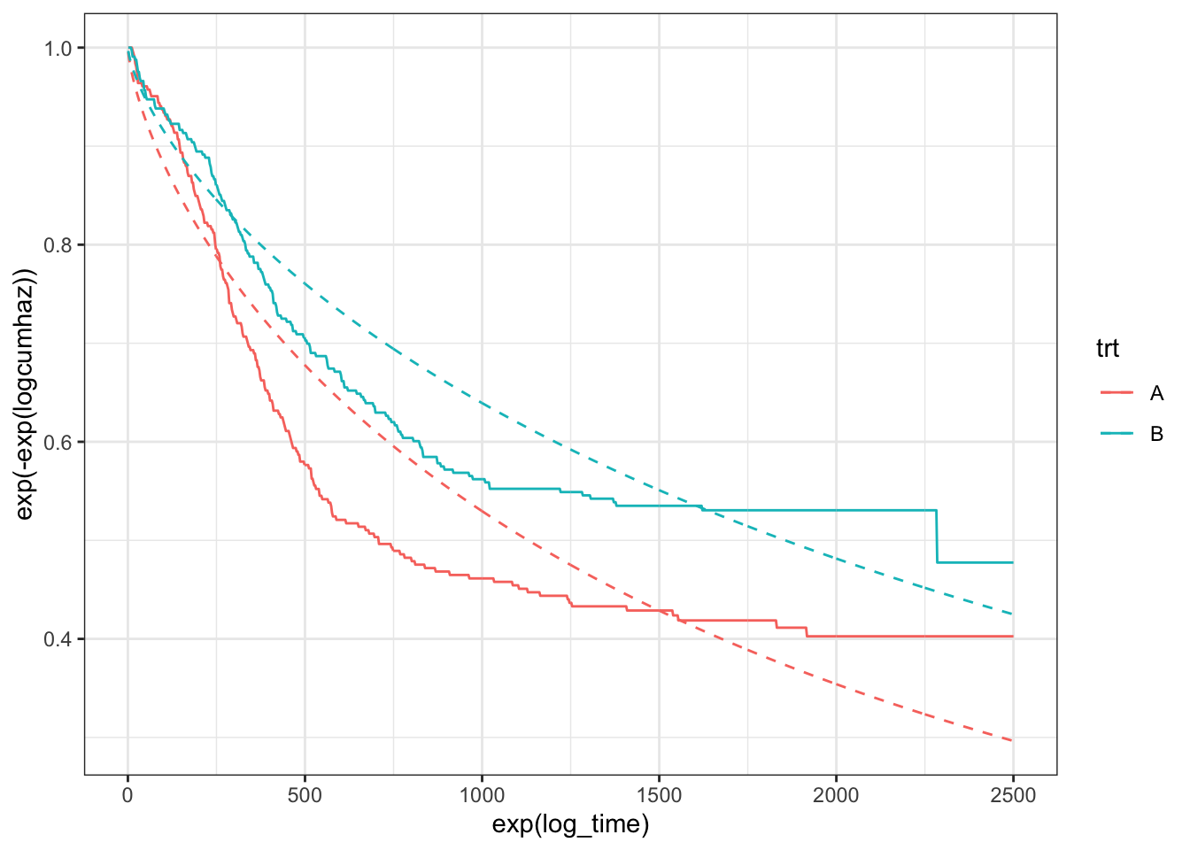

To improve the model, given this lack of linearity, it seems quite natural to change from

\[\log H(t;x) = a\log t - a\log(b) - a x^T\gamma\]

to

\[\log H(t;x) = s(\log t) + x^T\beta\]

where \(s(\log t)\) is a natural cubic spline function of (log) time. One can make the model more/less flexible by choosing a large/small number of knots. By default, the knots are placed at quantiles of the uncensored event times. How many knots are required? I don’t really have a good answer for this: one or two. At most, three? In this example, I’m using two inner knots, placed at 33% and 66% of the uncensored event times (indicated by vertical lines):

fit_spline_2 <- flexsurvspline(Surv(futime, death) ~ trt, 
                               data = myeloid,
                               k = 2,
                               scale = "hazard")

spline_2_sum <- summary(fit_spline_2, t = t_seq, type = "cumhaz")

df2 <- cbind(df,
      data.frame(logcumhaz_s2 = log(c(spline_2_sum$`trt=A`["est"]$est,
                                  spline_2_sum$`trt=B`["est"]$est))))

ggplot(data = df2,
       mapping = aes(x = log_time,
                     y = logcumhaz,
                     colour = trt)) +
  geom_line() +
  geom_line(mapping = aes(x = log_time,
                          y = logcumhaz_s2,
                          colour = trt),
            linetype = 2) +
  theme_bw() +
  scale_x_continuous(limits = c(2,8)) +
  scale_y_continuous(limits = c(-6,0)) +
  geom_vline(xintercept = fit_spline_2$knots)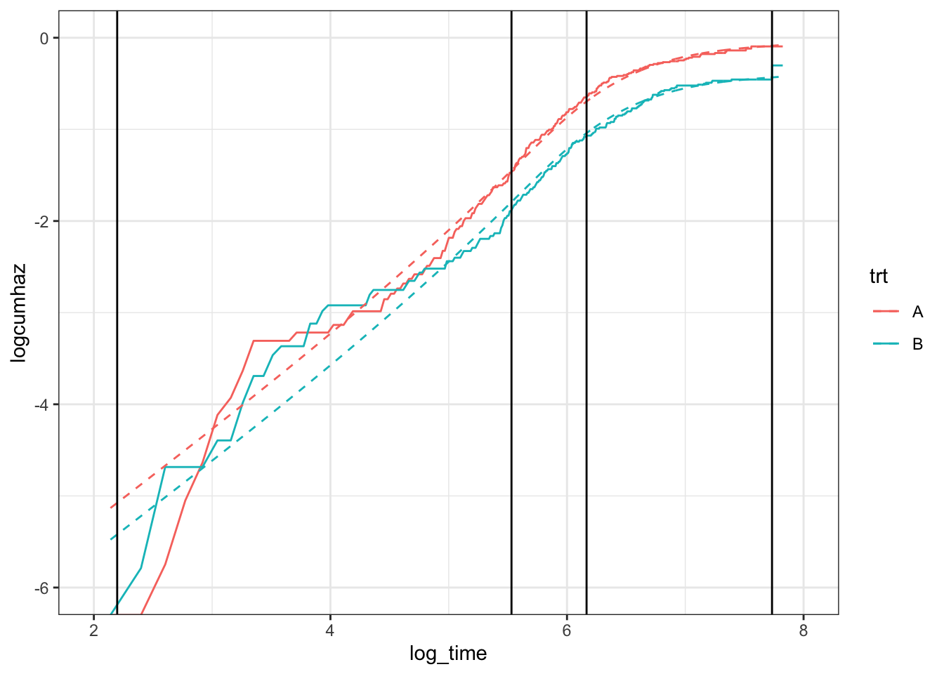

This looks a lot better, and we can see the improvement in the survival curves:

ggplot(data = df2,
       mapping = aes(x = exp(log_time),
                     y = exp(-exp(logcumhaz)),
                     colour = trt)) +
  geom_line() +
  geom_line(mapping = aes(x = exp(log_time),
                          y = exp(-exp(logcumhaz_s2)),
                          colour = trt),
            linetype = 2) +
  theme_bw()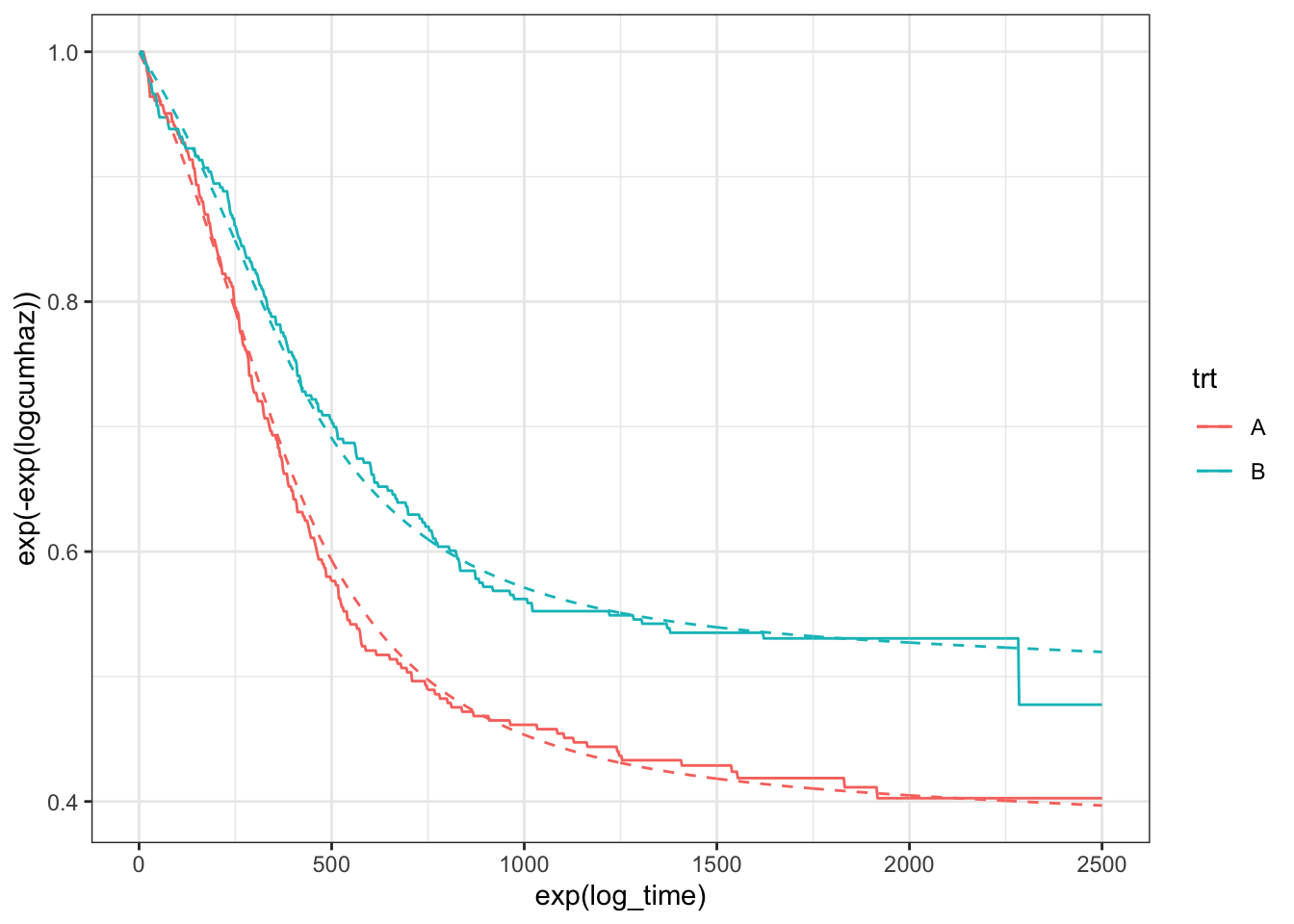

From Cox regression to Weibull regression.

If we start out from Cox regression

\[h(t;x)=h_0(t)\exp(x^T\beta)\]

this means that

\[\log H(t;x) = \log H_0(t;x) + x^T\beta\]

We estimate the parameters \(\beta\) from the partial likelihood, and don’t estimate \(\log H_0(t;x)\). So \(\log H_0(t;x)\) can be anything. However, with the flexsurvspline function, as long as we use enough knots, \(s(\log(t))\) can be more-or-less anything (smooth), so the two methods will give the same information about \(\beta\).

Conclusions

I can’t really see any reason not to switch from a Cox model to flexsurvspline. You don’t lose anything in terms of inference on \(\beta\), only gain a nice estimate for the baseline hazard. Also, inference is all based on maximum likelihood. No special theory required.

From the other side, if you start out from Weibull regression, and then realise that Weibull is the wrong model, you don’t have to think too hard about how to choose a better model, you know that flexsurvspline will be good (assuming proportional hazards is correct: for non-proportional hazards you may have to think harder).

What can go wrong? In small sample sizes, I guess there could be issues with over-fitting if too many knots are chosen. But given a decent sample size, I can’t see any problems. I would be interested to see a \(\log H_0(t;x)\) that is highly wiggly – doesn’t seem likely in practice.